External Flow
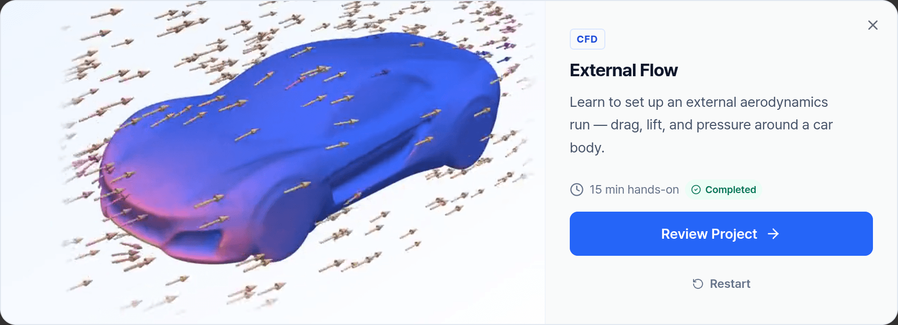
In this tutorial you simulate the airflow around a car driving on the road. You set the fluid box and the wind speed, run the case, read velocity, turbulence, and pressure in the results, and finish with the drag and lift numbers in the report.
Duration: 15 min. Sample model: a prepared car body whose surface is already wrapped, so it is ready to mesh. A new project lists it as Car.stl. The project in the figures is an earlier one and lists it as car_cfd_healed_wrap.
How the tutorial works
Open Tutorials in the dashboard and start External Flow. A guide card walks you through the stages Geometry, Model, Physics, Solve, Results, and Report.
- A page's tasks tick themselves off when you do them. Next unlocks once all of them are done.
- Only the controls the current task needs respond to clicks.
- Click a task to see where it is on screen.
Run Simulation in a tutorial submits no job. After about 3 seconds it opens a result computed in advance with these same settings. In your own projects, Run creates the mesh and solves the flow, and the values follow your inputs.
Geometry
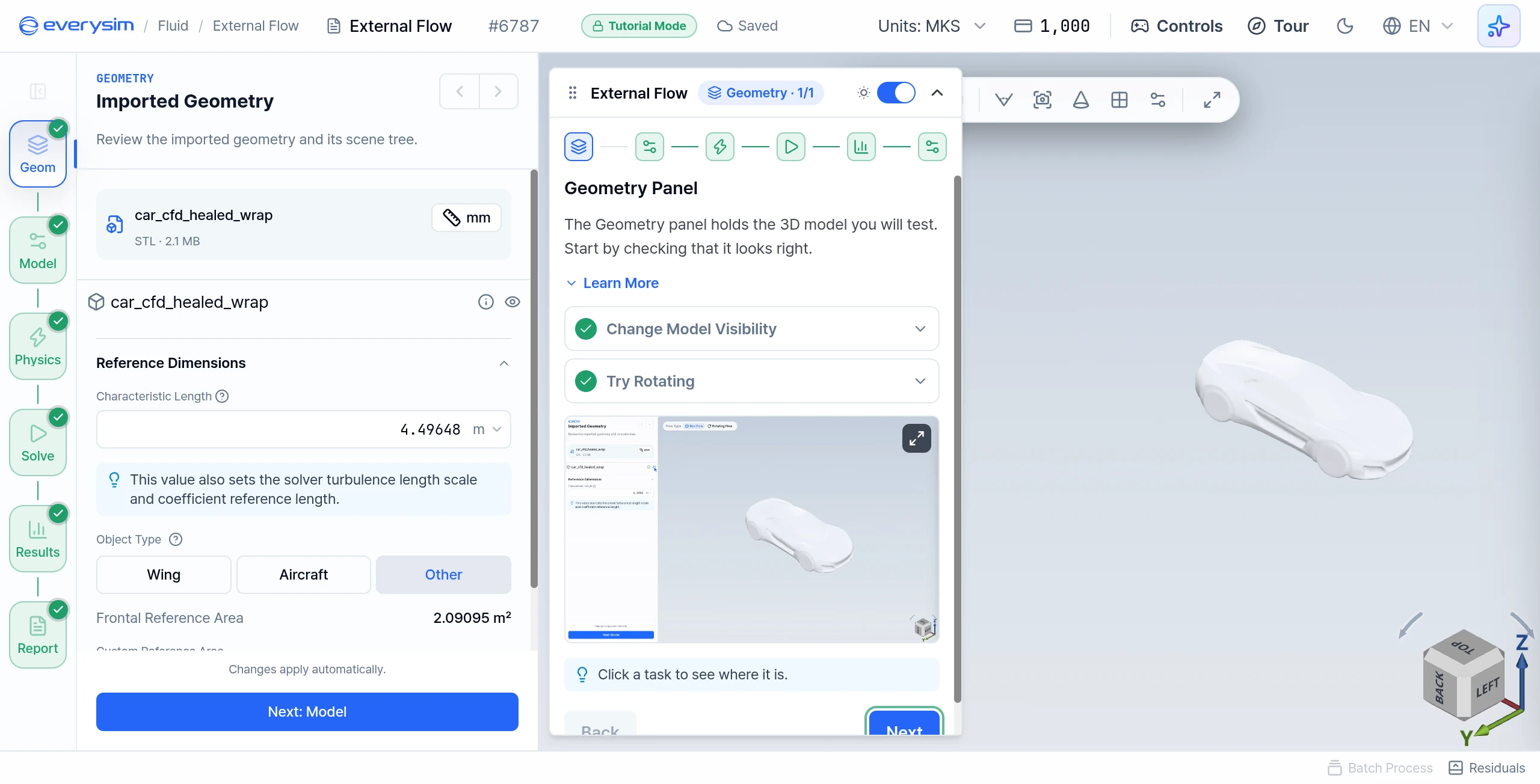
Geometry Panel
The Geometry panel holds the 3D model. Here you can look at its parts, show or hide them, and enter information about the geometry.
- Change Model Visibility: toggle the eye icon to hide the model, then show it again.
- Try Rotating: drag in the 3D viewport to rotate the model.
- Click Next.
Model
Fluid Box Size
The fluid domain sets the size of the region the simulation runs in. Too small a box distorts the result. Too big a box only adds run time.
- Interact with the Canvas: hover over the box until its handles appear, then drag one to see the size change. A box you resize becomes your own, under Custom Box Dimensions.
- Choose a Fluid Box Size: under Fluid Box Size, choose Medium, the size recommended for an uploaded model. Small is the fastest and Large is the most accurate.
- Click Next.
With Medium, the Domain Size reads 58.454 × 28.998 × 28.232 m.
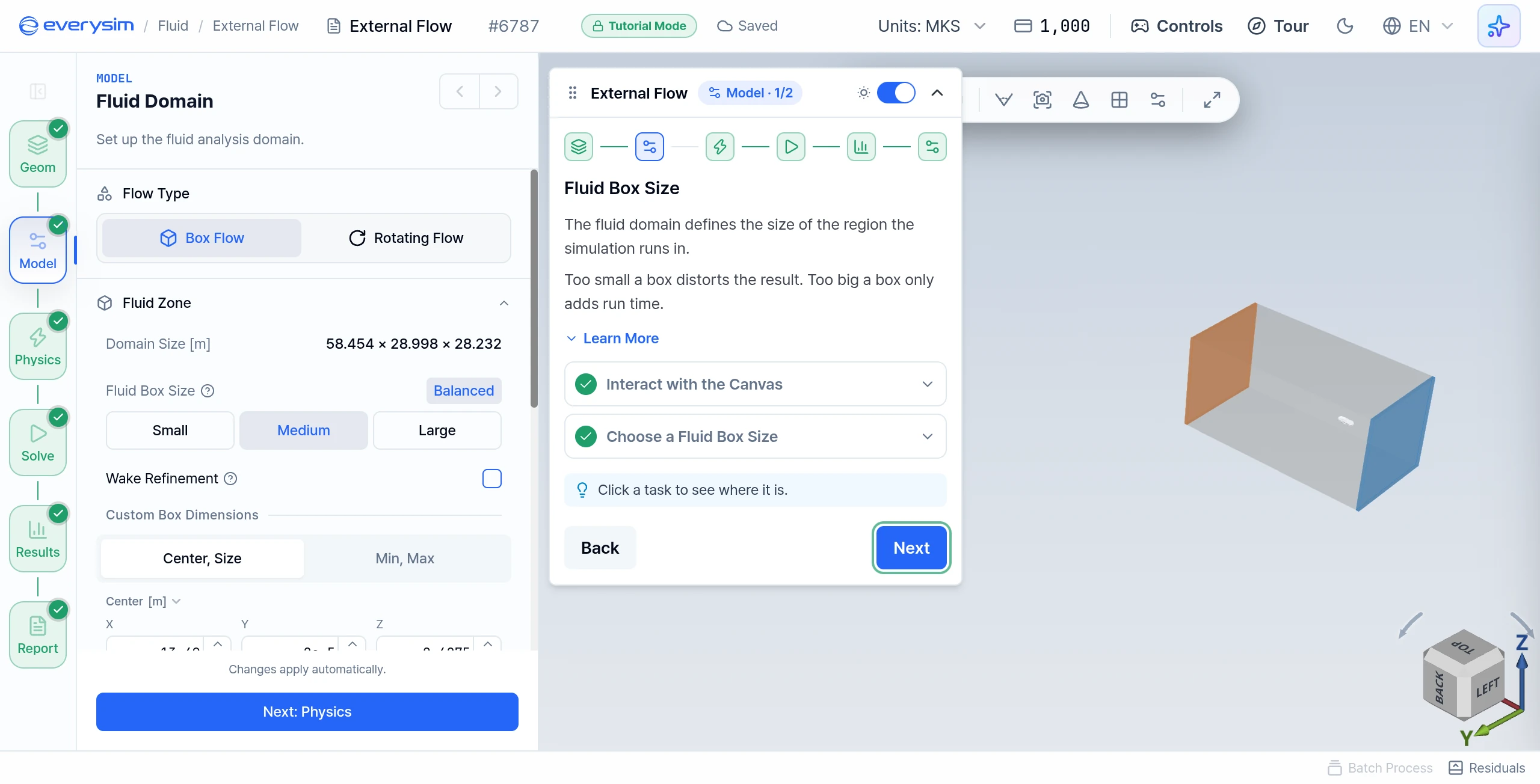
To size the box by numbers, open Custom Box Dimensions, choose Center, Size or Min, Max, and edit the X, Y, and Z fields.
Fluid Properties
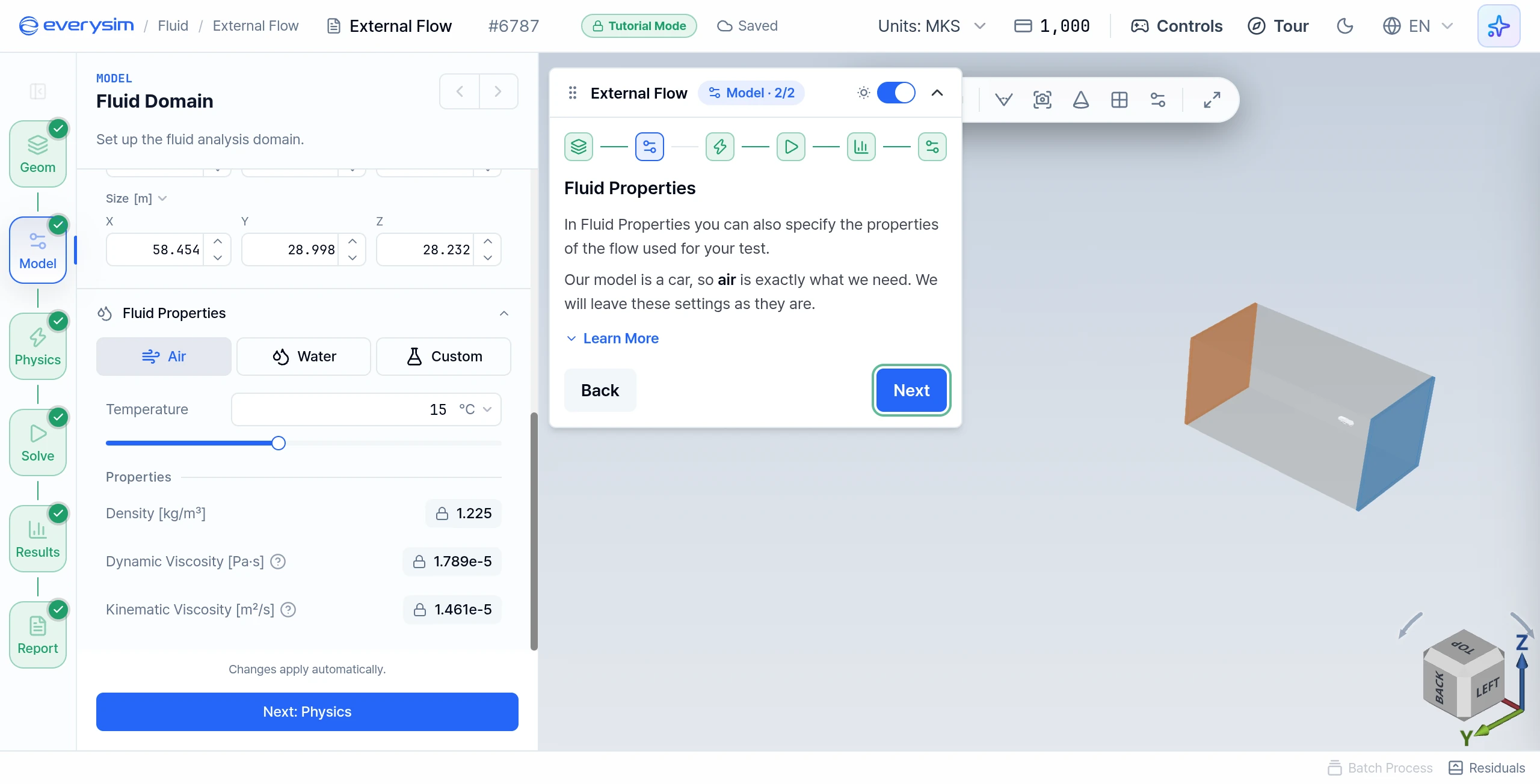
There is nothing to change on this page. The model is a car, so Air stays selected. Look over the values and click Next. In your own project you can switch to the fluid you need, such as Water.
Physics
Physics Panel
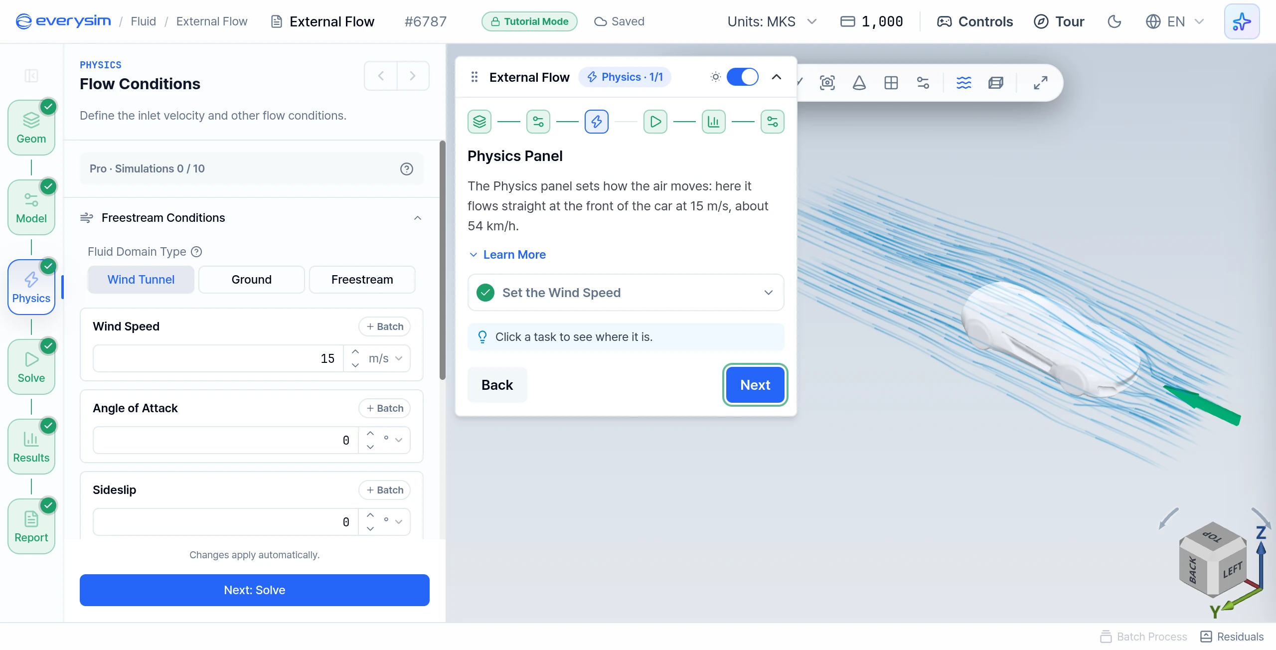
We simulate a car driving forward. In the simulation the car stays still and the air moves instead, and the effect on the car is the same.
- Set the Wind Speed: in Wind Speed, type
15and press Enter. That is 15 m/s, about 54 km/h, flowing straight at the front of the car. - Leave Angle of Attack at its default
0°. It tilts the oncoming air up or down, and a car meets the air level. - Click Next.
Solve
Solve Panel · Accuracy
Accuracy controls how finely the mesh divides the space into cells. Higher levels take more time and credits. Mesh Settings stays on Auto · accuracy-based.
- Set Accuracy to 4: move the Accuracy slider to
4, a good balance of precision and cost for this case. - Click Next.

Solve Panel · Acceleration
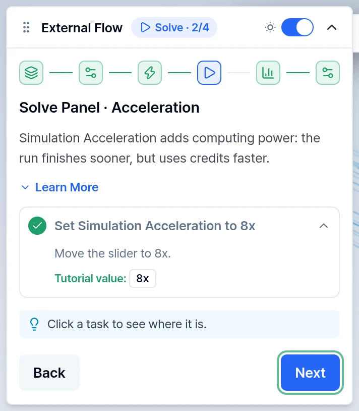
Simulation Acceleration adds computing power. The run finishes sooner but uses credits faster. It changes only the speed, not the quality of the results.
- Set Simulation Acceleration to 8x: move the slider to
8x. - Click Next.
Run Simulation
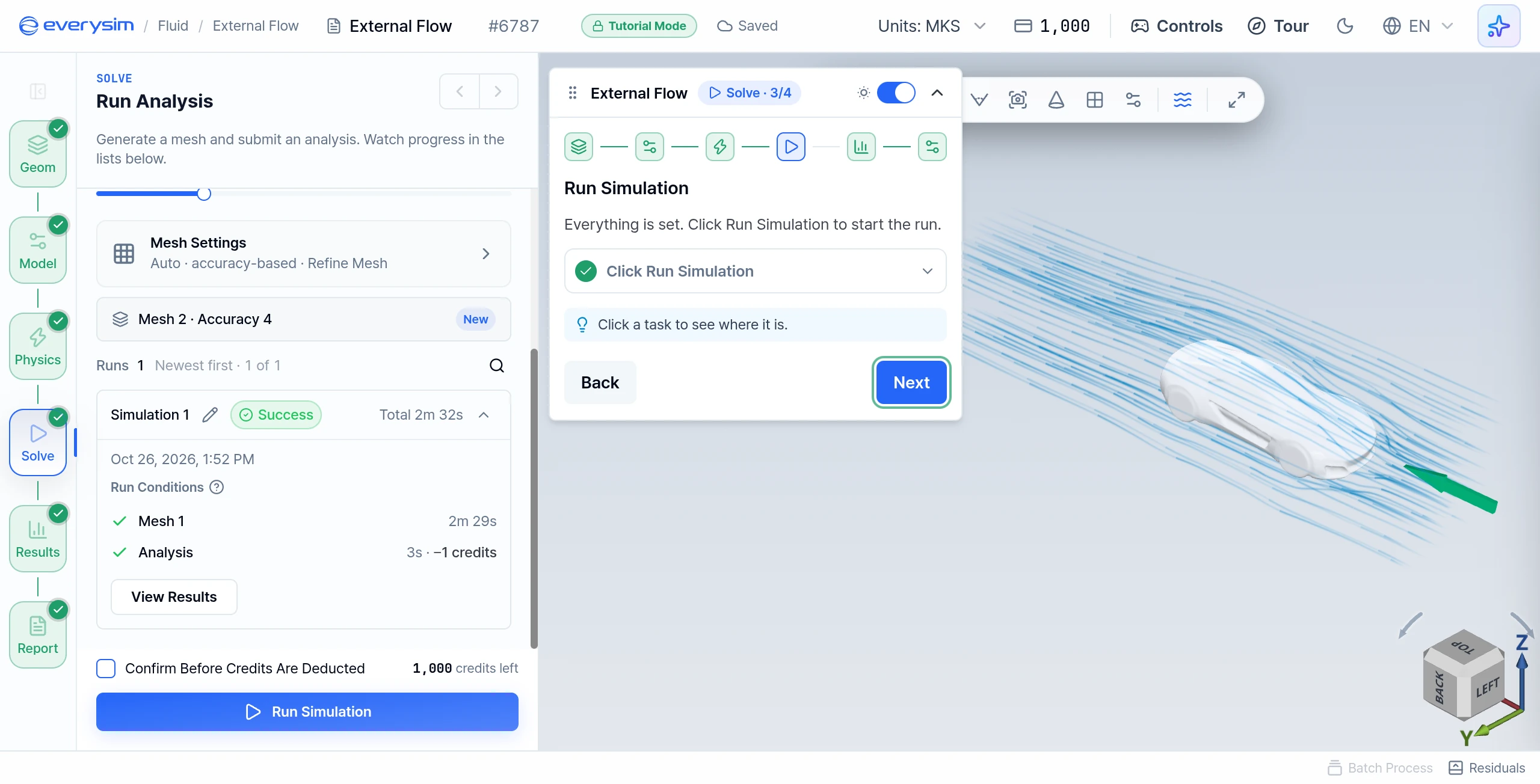
Click Run Simulation at the bottom of the Solve panel. If geometry data is still being prepared, wait for the button to become available.
Simulation Process
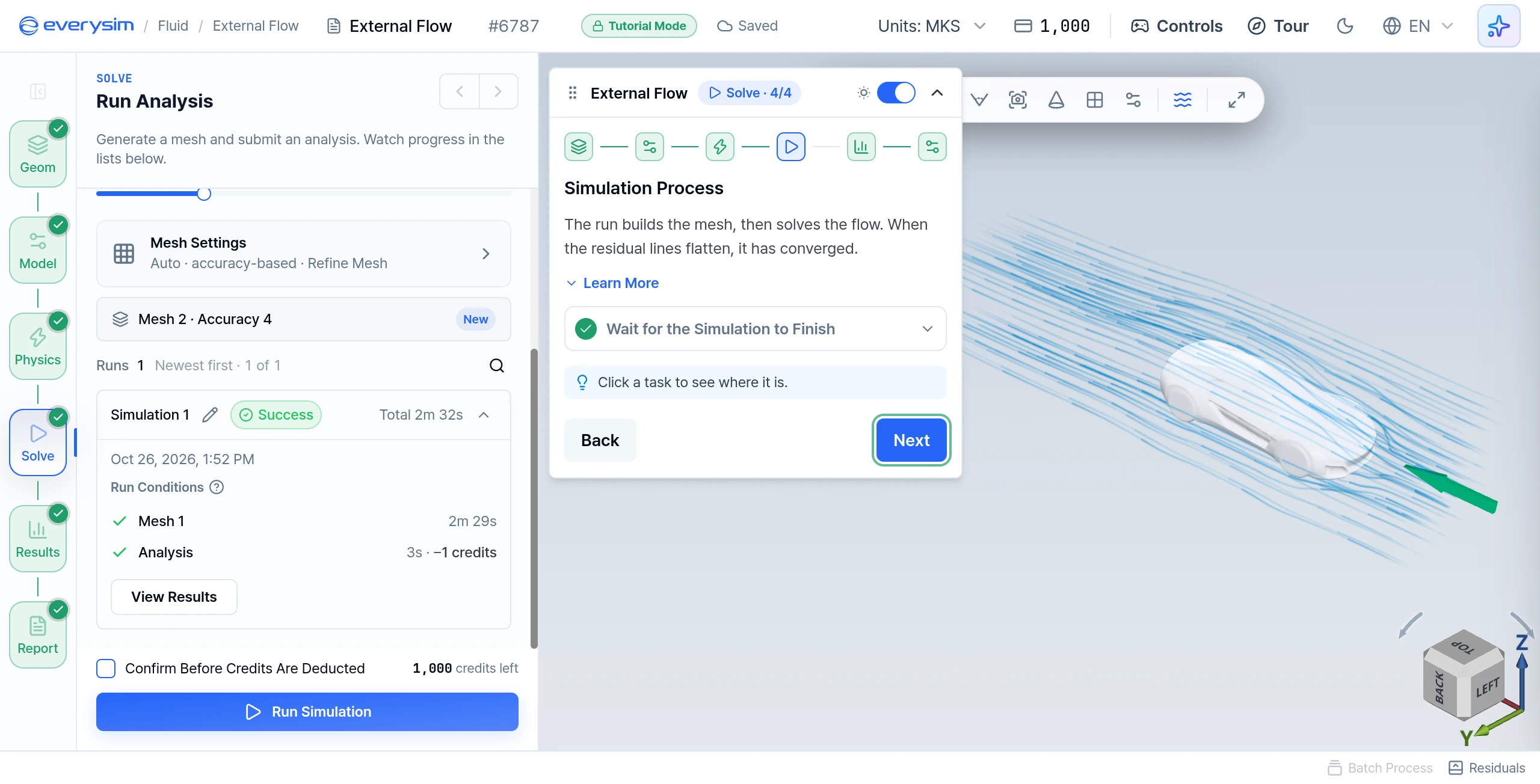
Wait for the Simulation to Finish. In a tutorial this takes about 3 seconds, and then the prepared result opens by itself.
In your own projects the run has two phases. Mesh splits the simulation space into small cells, and Analysis calculates the flow on them. Click Residuals in the status bar to open the chart: residuals are the calculation error still left, and when the lines go down and flatten, the solution has converged.
Results
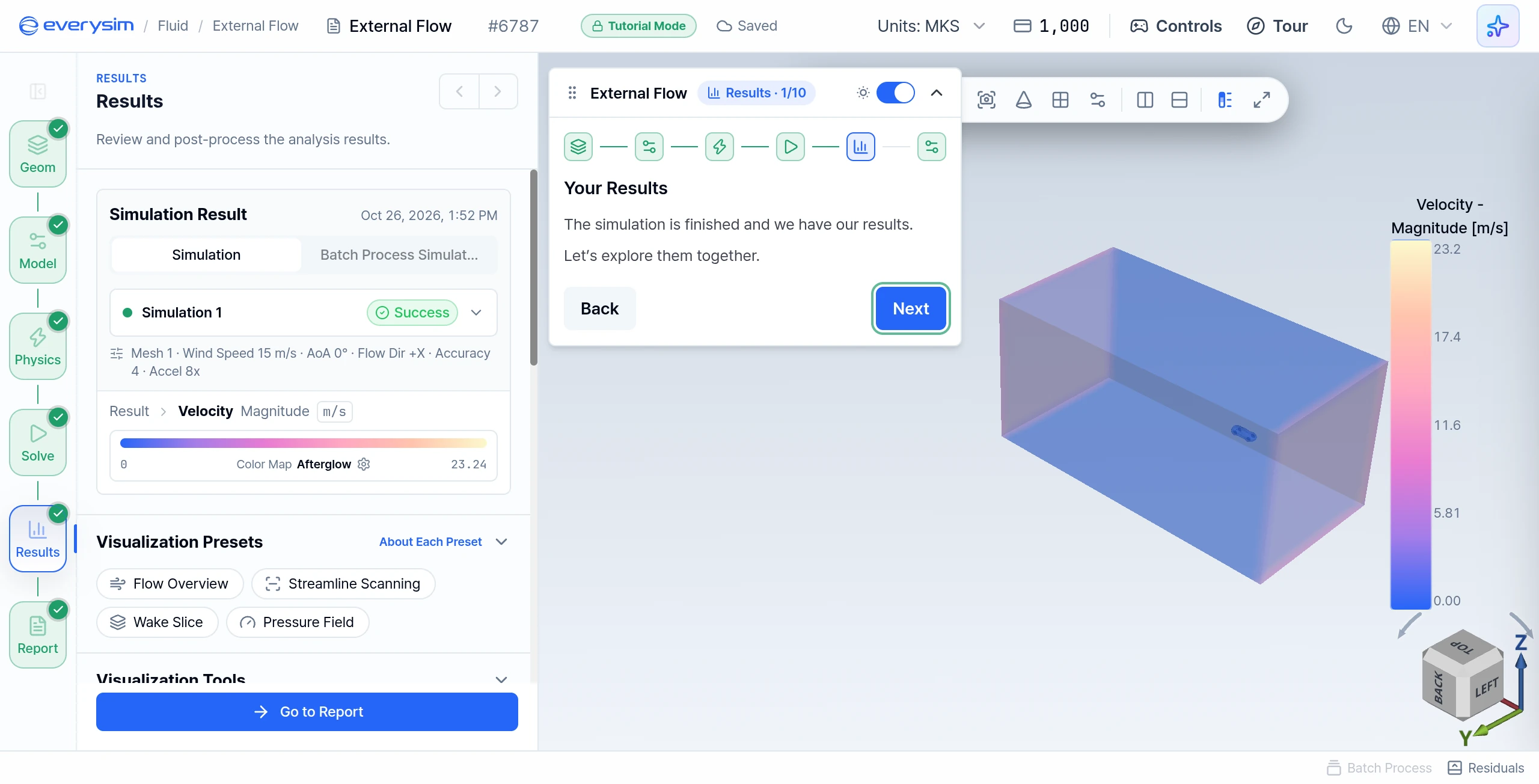
Your Results
The Results panel opens on the velocity magnitude, shown over the whole fluid domain. The simulation card sums up the run: Wind Speed 15 m/s, AoA 0°, Flow Dir +X, Accuracy 4, Accel 8x. Click Next.
Result Fields
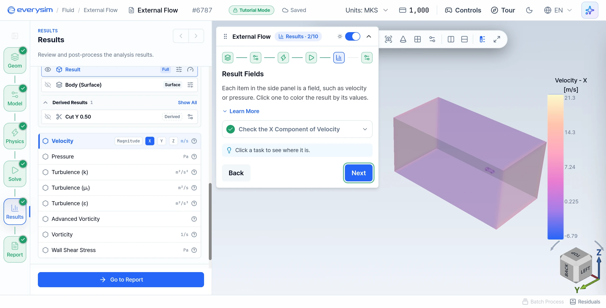
Each item in the side panel is a field. Clicking one colours the result by its values, and the colour bar shows which colour means which value.
- Check the X Component of Velocity: in Result Fields, click the X component on the Velocity row, because the flow direction is X.
- Click Next.
The list also offers Pressure, Turbulence (k), Turbulence (μₜ), Turbulence (ε), Advanced Vorticity, Vorticity, and Wall Shear Stress.
Cut Section
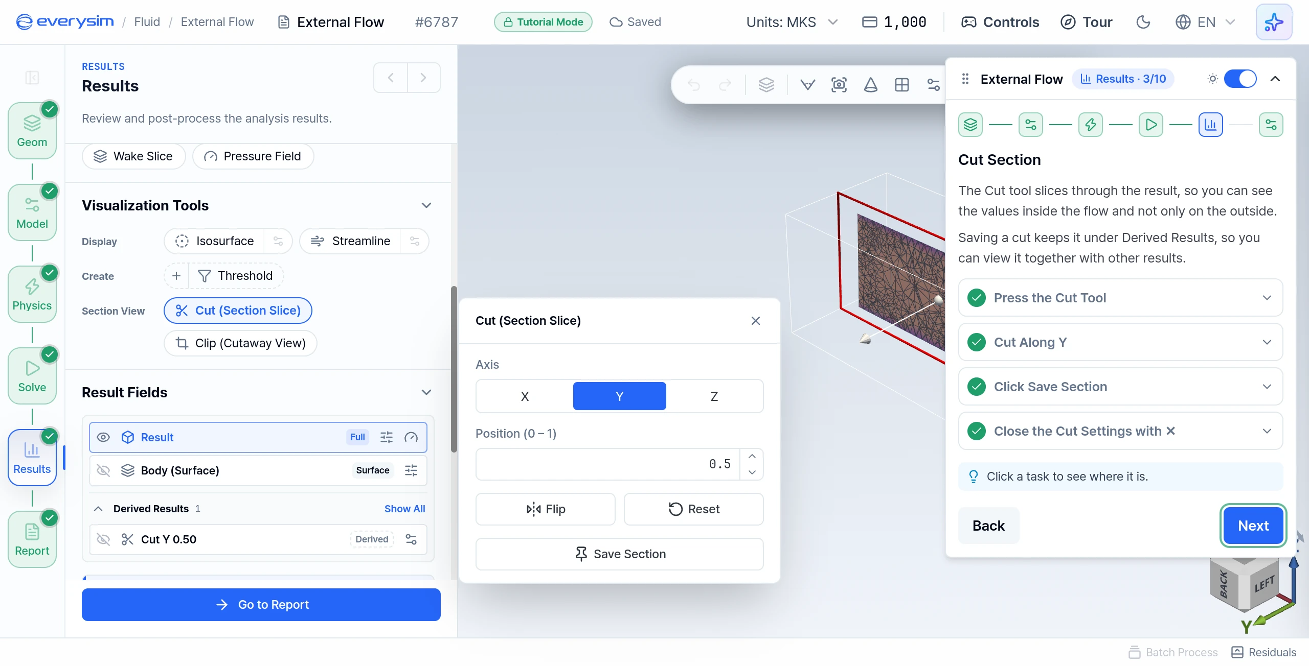
The Cut tool slices through the result, so you can see the values inside the flow. Saving a cut keeps it under Derived Results, where you can view it together with other results.
- Press the Cut Tool: under Visualization Tools, press Cut (Section Slice) in the Section View row. Its settings open beside the panel.
- Cut Along Y: choose Y as the axis, to see how the results are distributed along the flow direction.
- Click Save Section: this saves the cut under Derived Results as
Cut Y 0.50. - Close the Cut Settings with ✕: closing them turns the tool off. The adjusting plane goes away and only the saved cut is left.
- Click Next.
Camera View
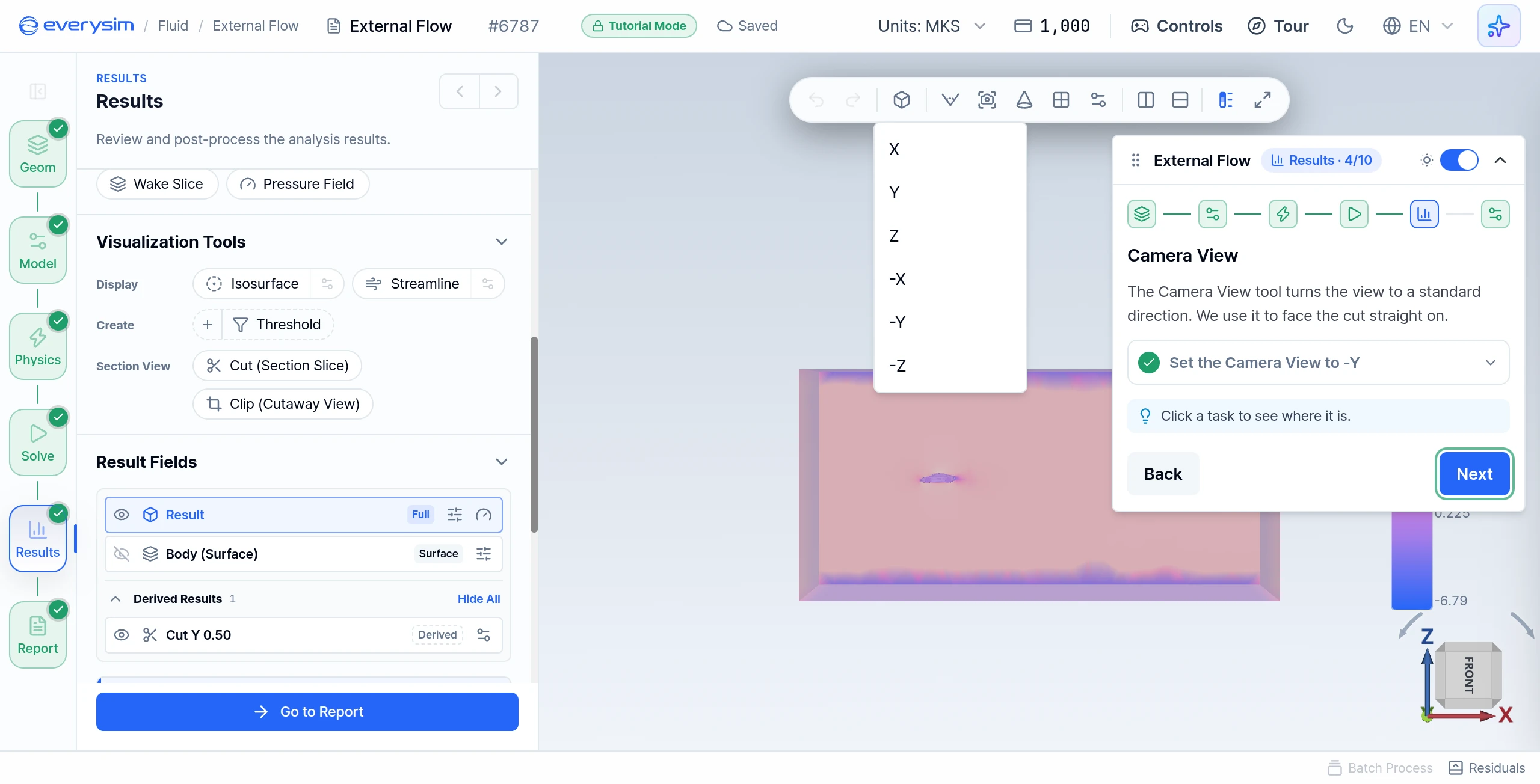
Set the Camera View to -Y: open Camera View in the toolbar above the viewport and choose -Y, so you face the cut straight on. Then click Next.
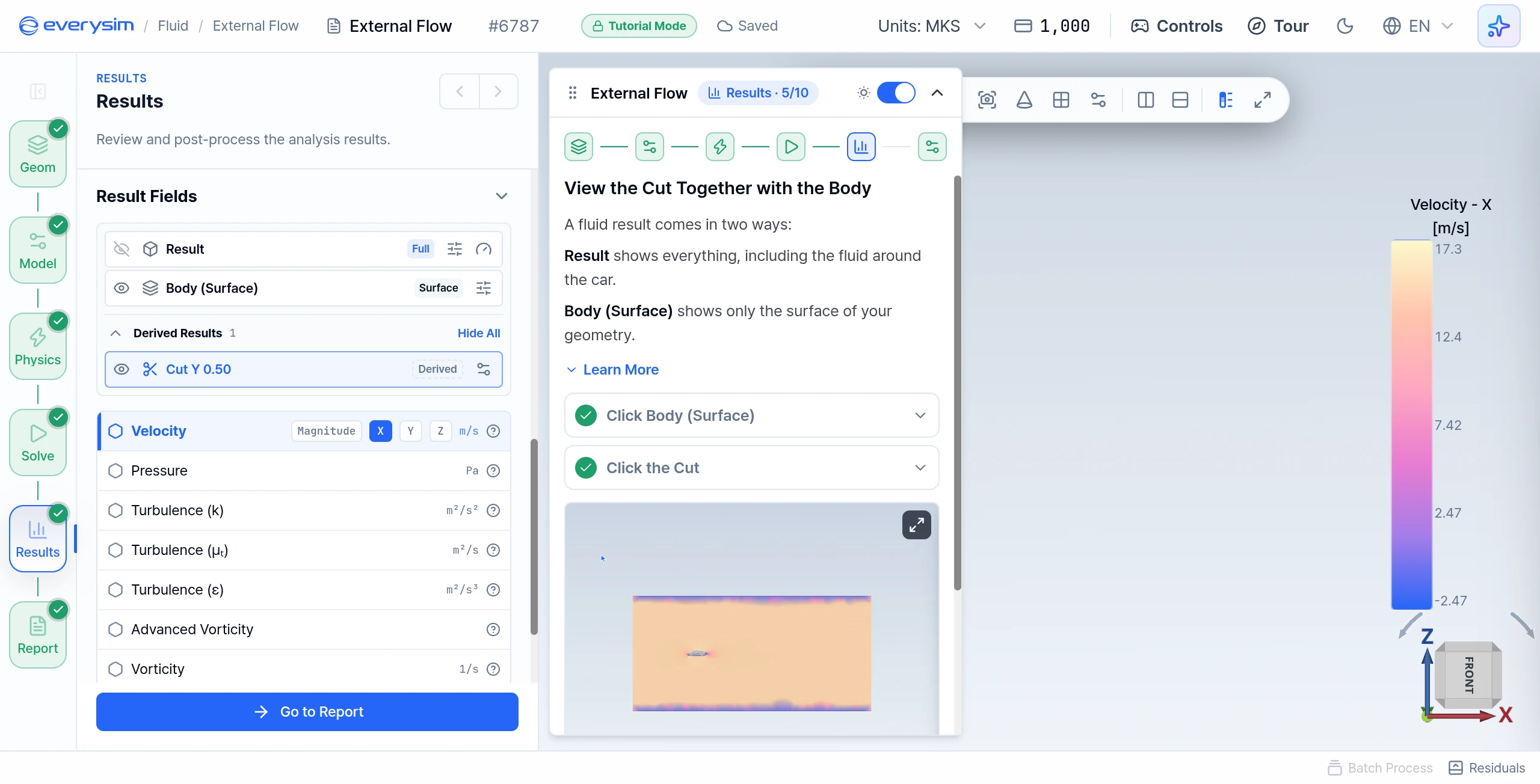
View the Cut Together with the Body
A fluid result comes in two ways. Result shows everything, including the fluid around the car. Body (Surface) shows only the surface of your geometry. A derived result, such as your cut, can be selected as well.
- Click Body (Surface): the fluid domain goes away and only the car surface stays.
- Click the Cut: click the cut's name under Derived Results. The cut is now selected, so the next field you choose shows on it.
- Click Next.
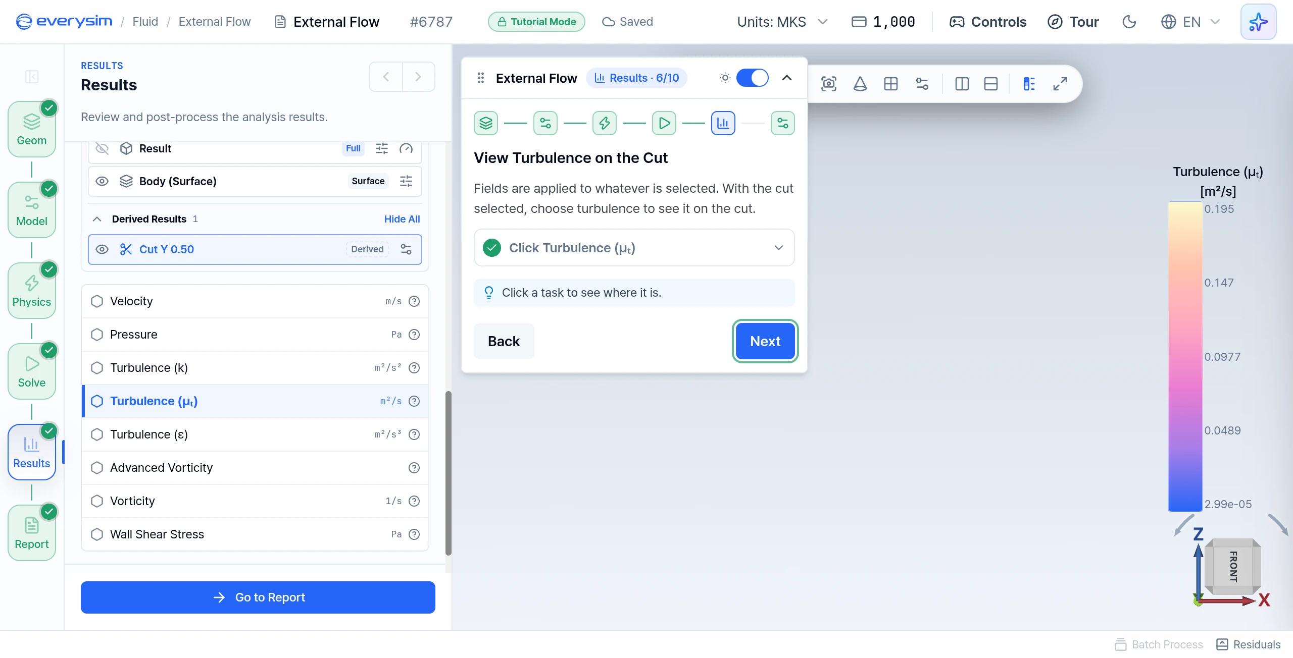
View Turbulence on the Cut
Fields apply to whatever is selected.
- Click Turbulence (μₜ): the cut shows how the flow changes as it passes the car, and the turbulent wake it leaves behind.
- Click Next.
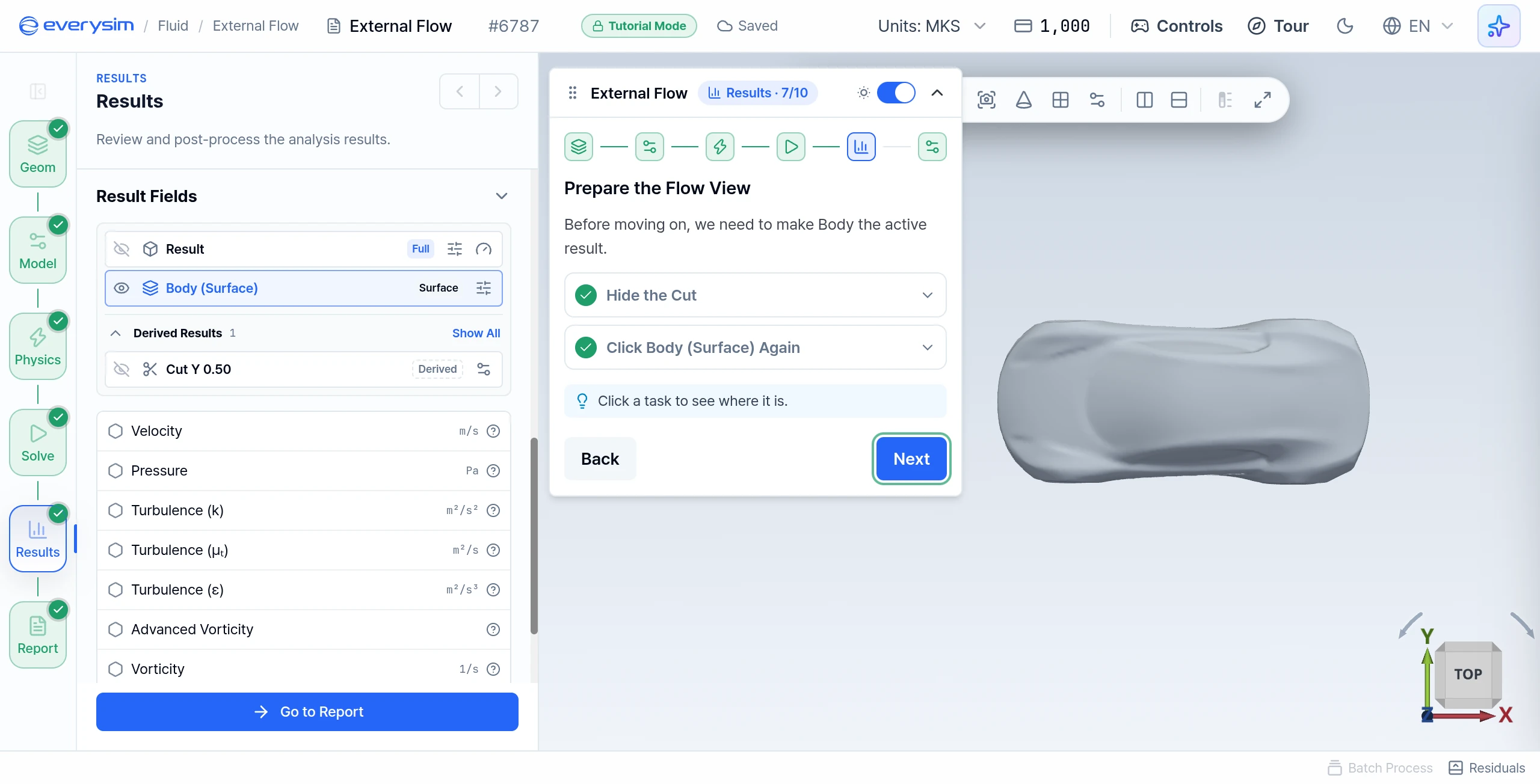
Prepare the Flow View
Before moving on, make the body the active result.
- Hide the Cut: click the eye on the cut's row.
- Click Body (Surface) Again: the body becomes the active result and the view turns to the Z direction.
- Click Next.
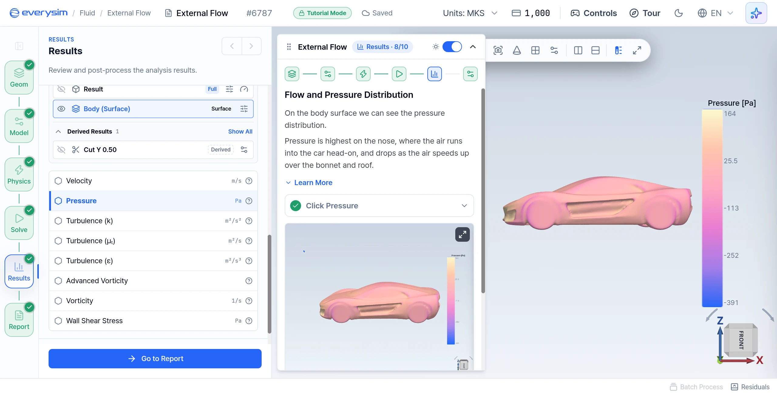
Flow and Pressure Distribution
When the air meets the car, it pushes on the surface. That push is pressure. It is highest on the nose, where the air runs into the car head-on, and drops as the air speeds up over the bonnet and roof.
- Click Pressure: the view turns to the side of the car. Compare the colours on the front with those over the roof. Scroll the mouse wheel over the viewport to zoom in.
- Click Next.
Streamline Animation
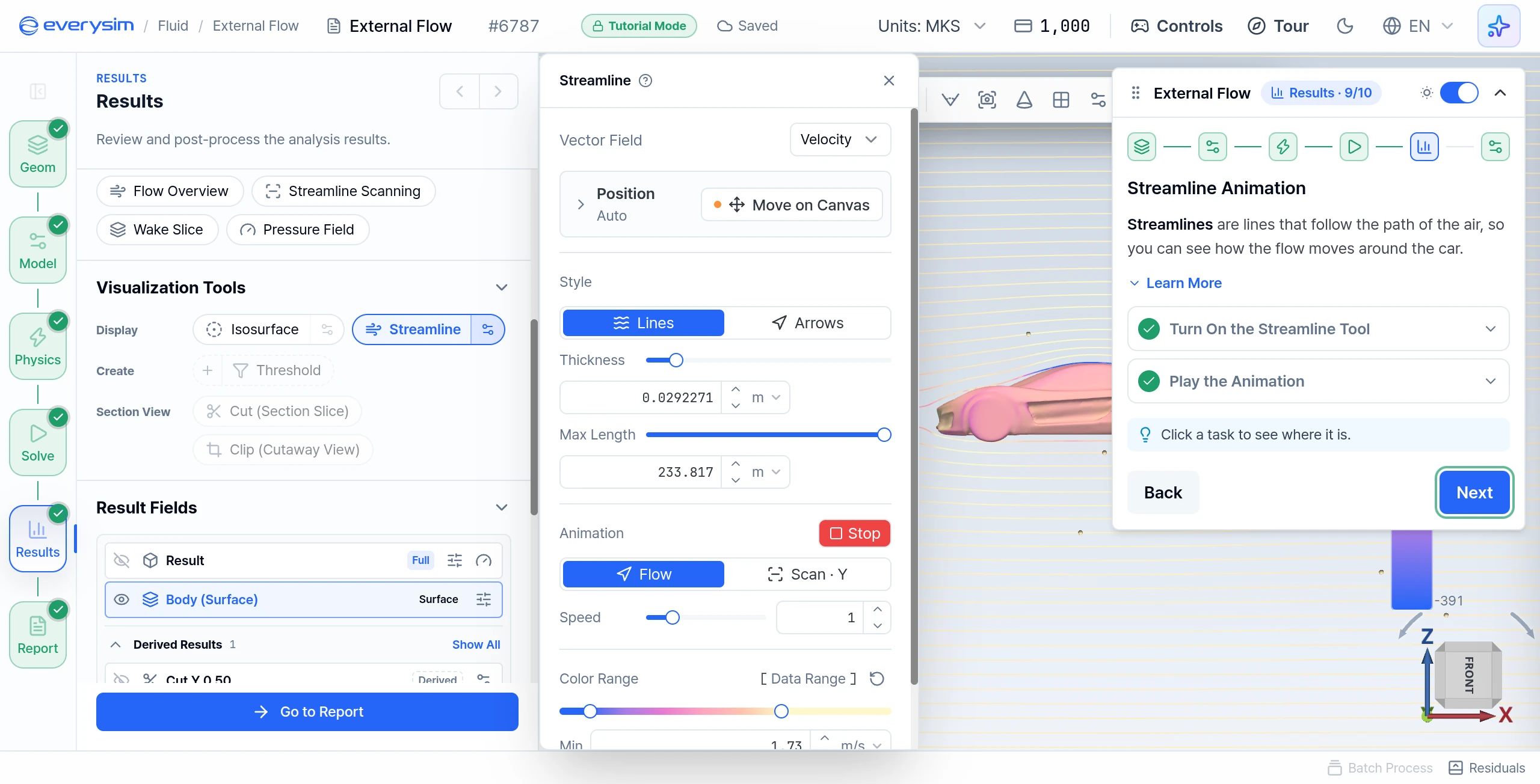
Streamlines follow the path of the air, so you can see how the flow moves around the car.
- Turn On the Streamline Tool: under Visualization Tools, switch on Streamline. Its settings open right away.
- Play the Animation: choose Lines or Arrows, then press Play in the Animation row.
- Click Next.
In your own projects you can also set the vector field, position, thickness, and maximum length here.
Report
Open the Report: a report is generated for every simulation and collects the key numbers in one place. Click Go to Report at the bottom of the panel.
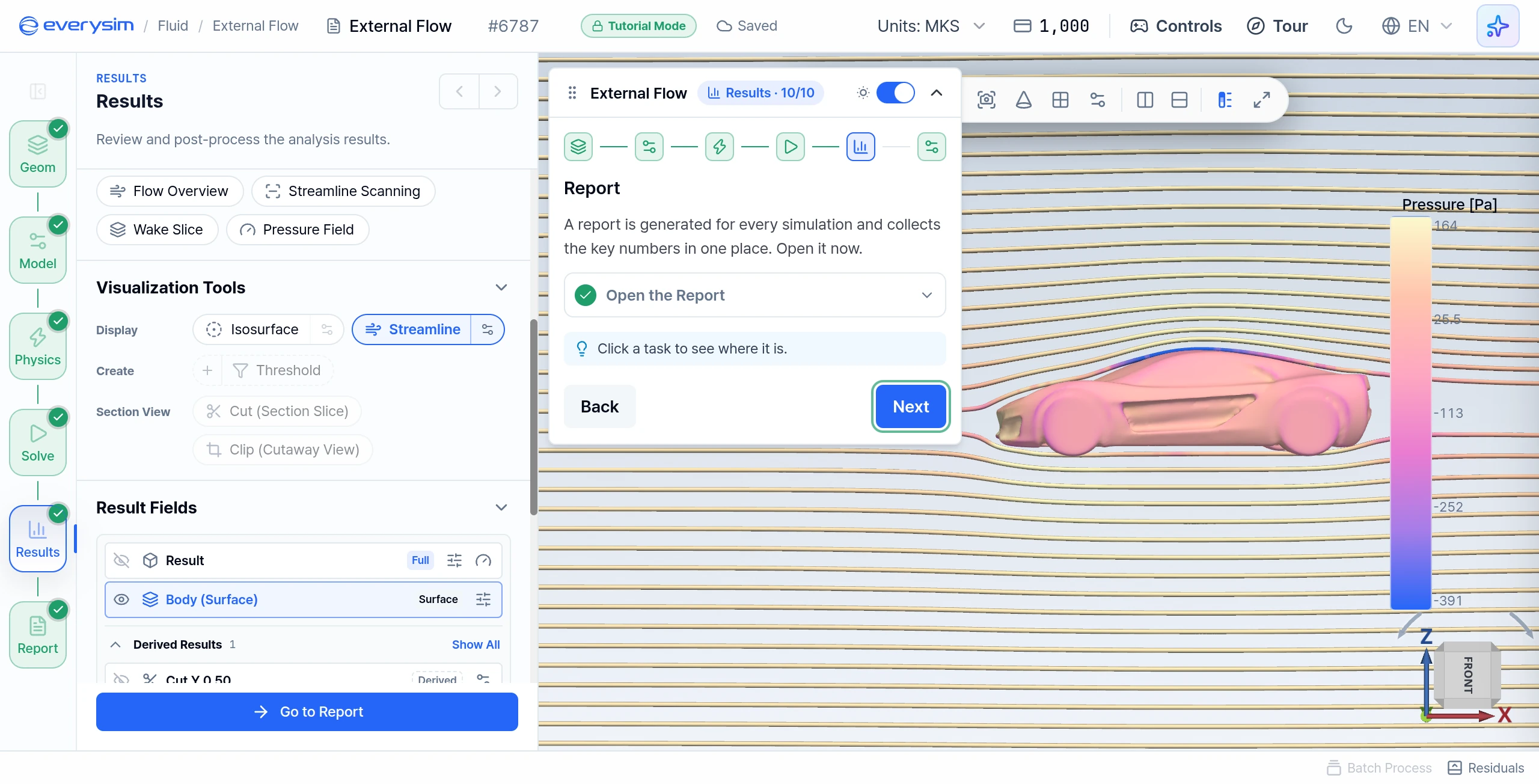
Report
Click Next to step through the sections. The last page has Finish instead of Next, and pressing it completes the tutorial.
Core Performance
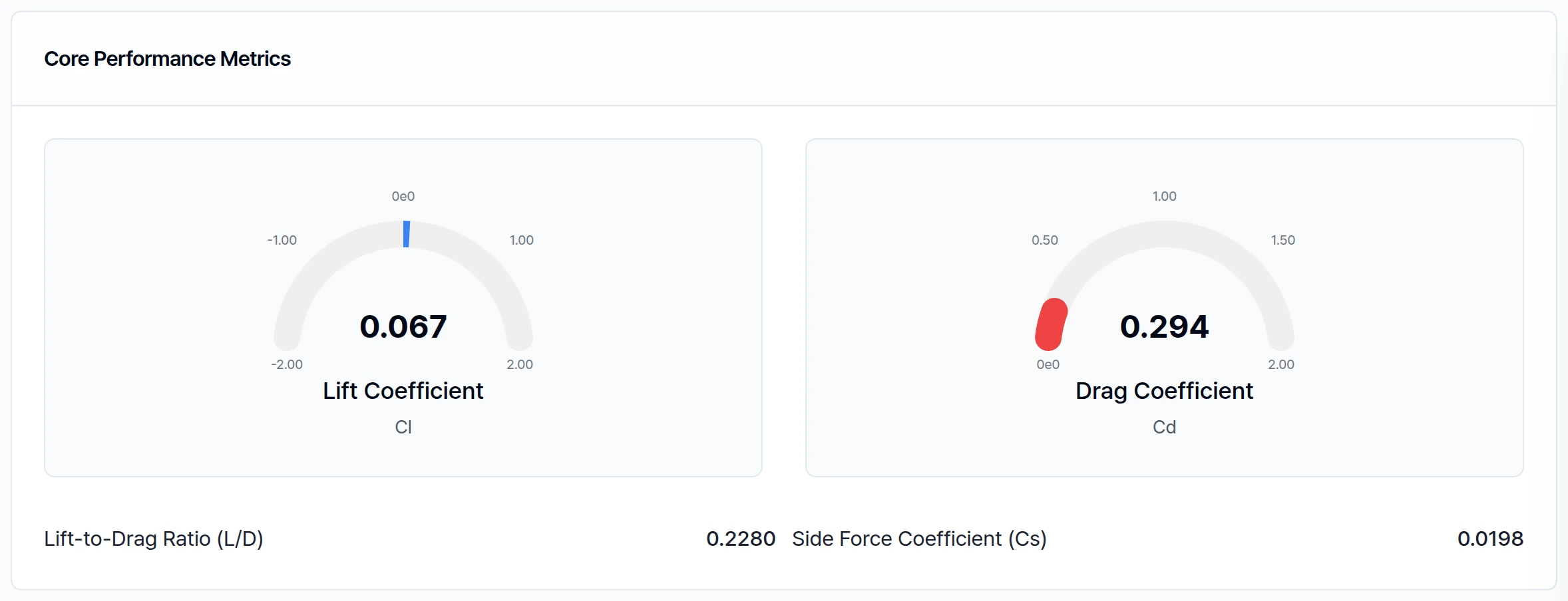
Drag holds the car back as it moves forward. The lower it is, the less energy the car needs at speed. Lift pushes the car up off the road and takes grip away from the tyres, so a road car wants little of it.
| Value | Result |
|---|---|
| Lift Coefficient (Cl) | 0.067 |
| Drag Coefficient (Cd) | 0.294 |
| Lift-to-Drag Ratio (L/D) | 0.2280 |
| Side Force Coefficient (Cs) | 0.0198 |
A drag coefficient of about 0.29 is in the usual range of a streamlined road car, and the lift is close to zero.
Conditions
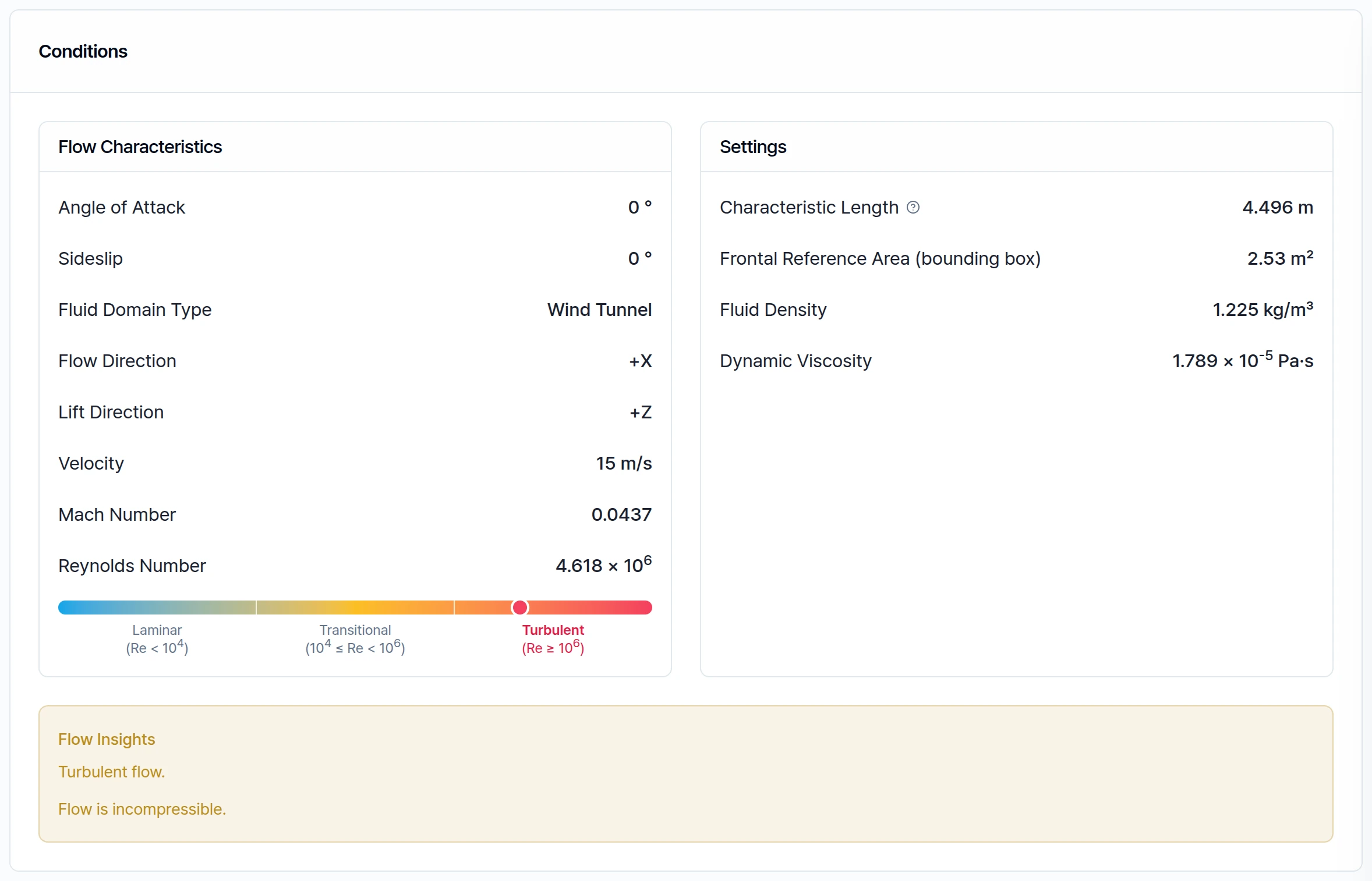
This section lists the conditions the result was calculated under. The Reynolds number tells you whether the flow is smooth or turbulent.
| Flow Characteristics | Settings | ||
|---|---|---|---|
| Angle of Attack | 0° | Characteristic Length | 4.496 m |
| Sideslip | 0° | Frontal Reference Area (bounding box) | 2.53 m² |
| Fluid Domain Type | Wind Tunnel | Fluid Density | 1.225 kg/m³ |
| Flow Direction | +X | Dynamic Viscosity | 1.789 × 10⁻⁵ Pa·s |
| Lift Direction | +Z | ||
| Velocity | 15 m/s | ||
| Mach Number | 0.0437 | ||
| Reynolds Number | 4.618 × 10⁶ |
Flow Insights reads: turbulent flow, and the flow is incompressible.
Force Distribution
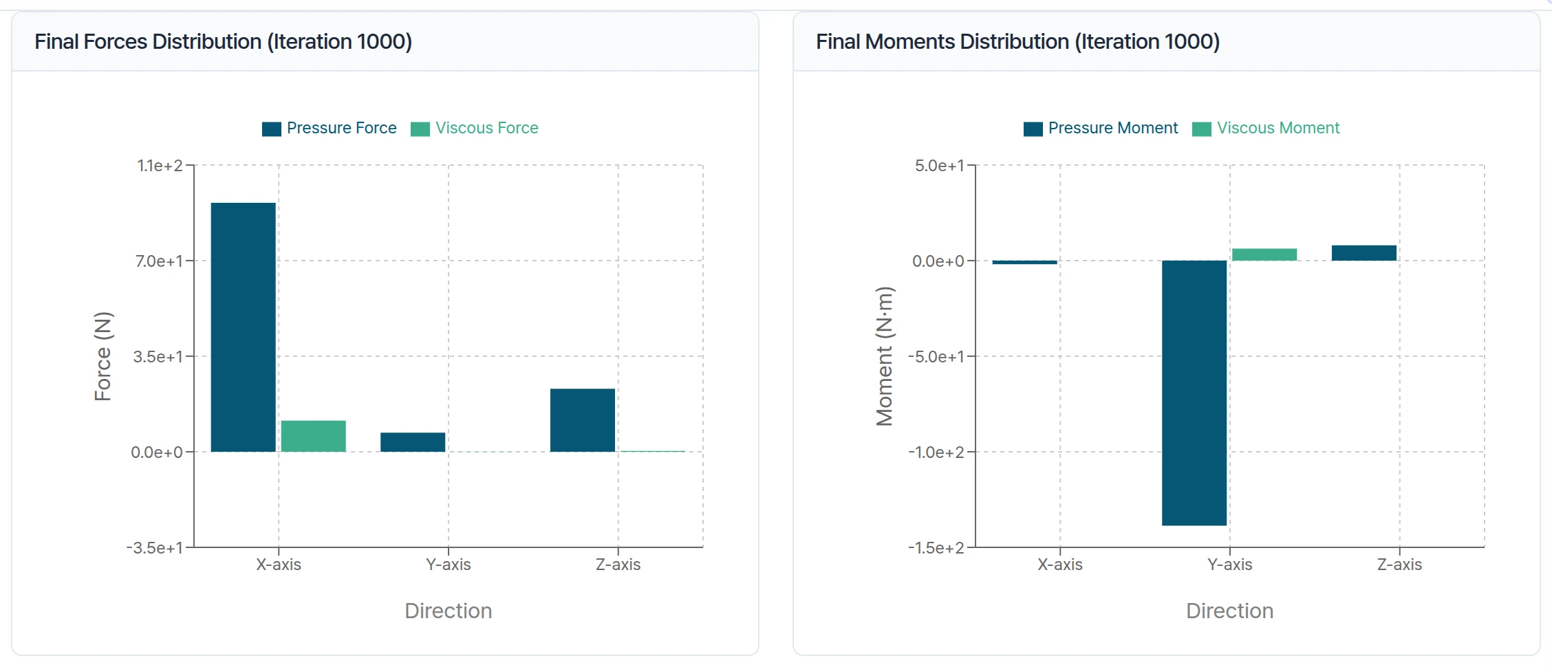
Pressure force comes from the air pushing on the surface. Viscous force comes from the air rubbing along the surface, like friction. The bar charts show, at the final iteration (1000), in which direction each force and moment is highest.
Convergence Graph
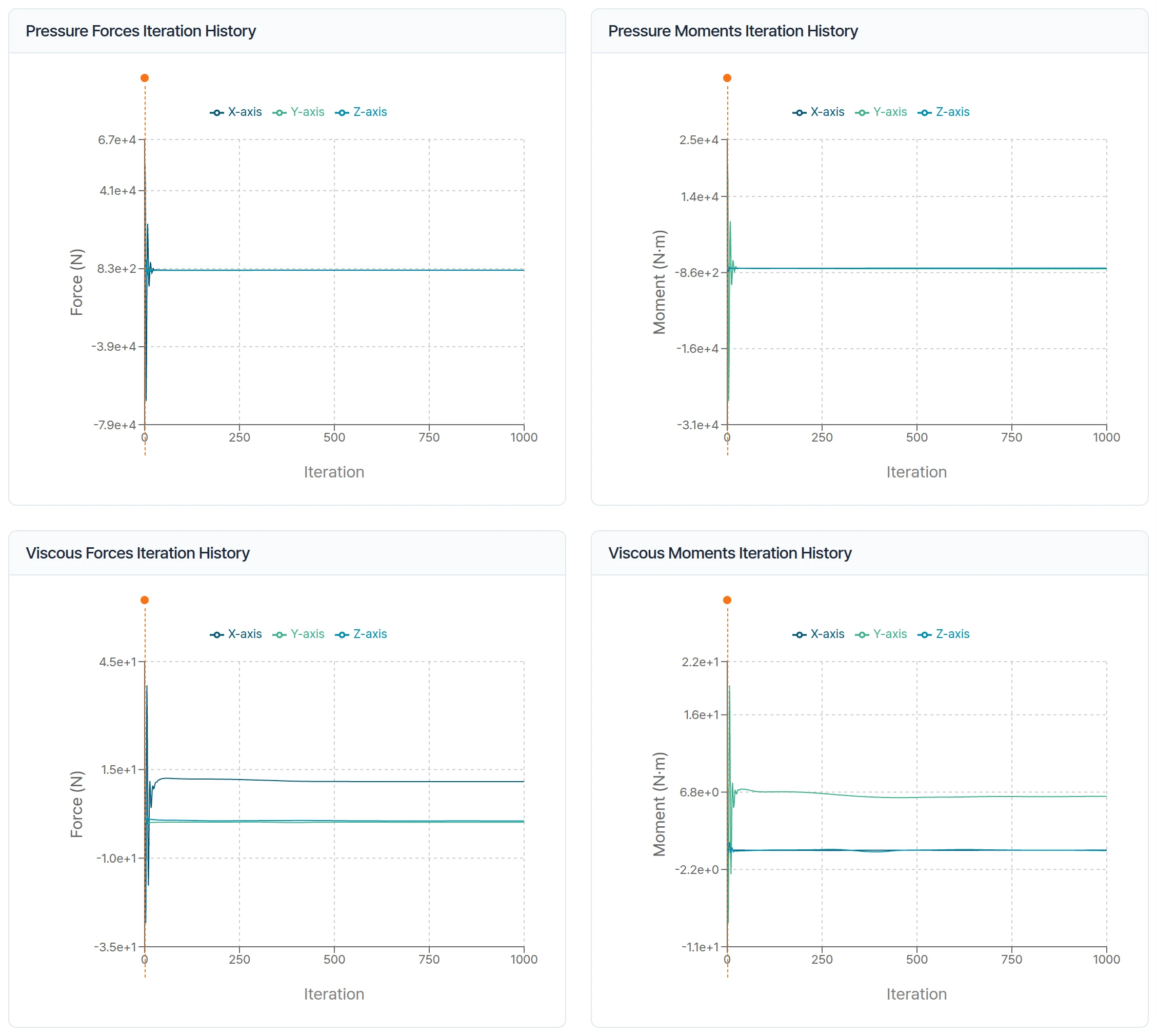
These graphs show how the calculated forces and moments changed while the simulation ran. The values move a lot at the start, and in a good simulation they settle so the line becomes almost flat. Here the drag has settled. The lift still drifts a little at the end, and a longer run would pin it down more closely.
Press Finish to complete the tutorial.
Need Assistance or Have Questions?
Frequently Asked Questions: FAQ Link
Support Inquiries: support@everysim.io