Transient Structural
This tutorial tests how a clevis pin assembly responds to a short, sudden push. You assign carbon steel, hold both support blocks by their undersides, apply a pulsed force to one block, then read how displacement and stress change over time. With no damping, the curves keep oscillating after the pulse ends. It takes about 25 minutes.
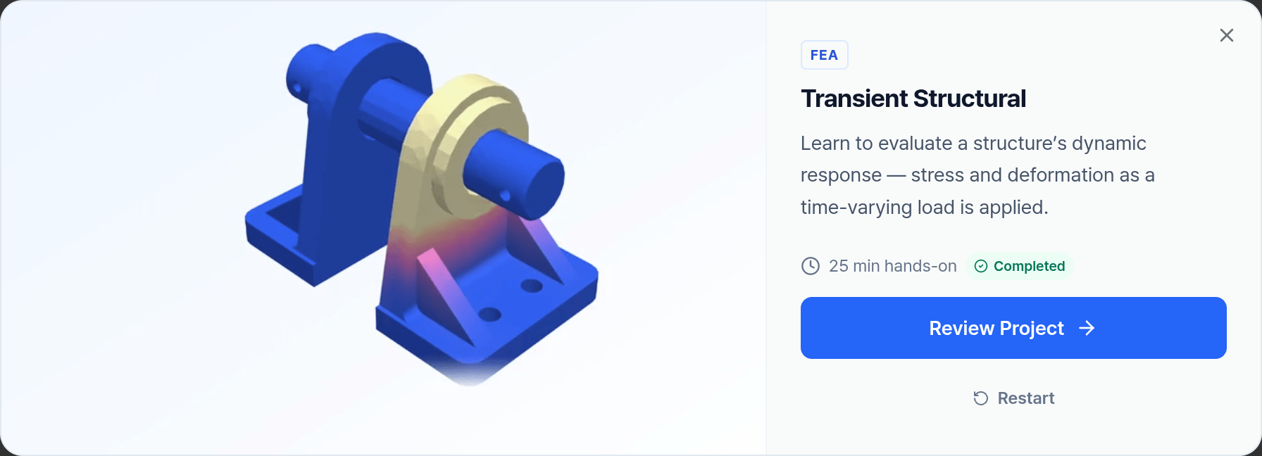
Start it from Tutorials in the dashboard. A guide card leads you through each page. Only the control a task highlights accepts clicks, and Next unlocks once the page's tasks are ticked. The project uses mm-t-s units: lengths in mm, stress in MPa, force in N.
What you will learn
- Assign one material to several parts with Select Unassigned Elements.
- Pick two faces at once with Shift.
- Define a pulsed load and read its load profile.
- Understand total time, time step and Rayleigh damping.
- Read peak values and time histories in the report.
1. Geometry Panel
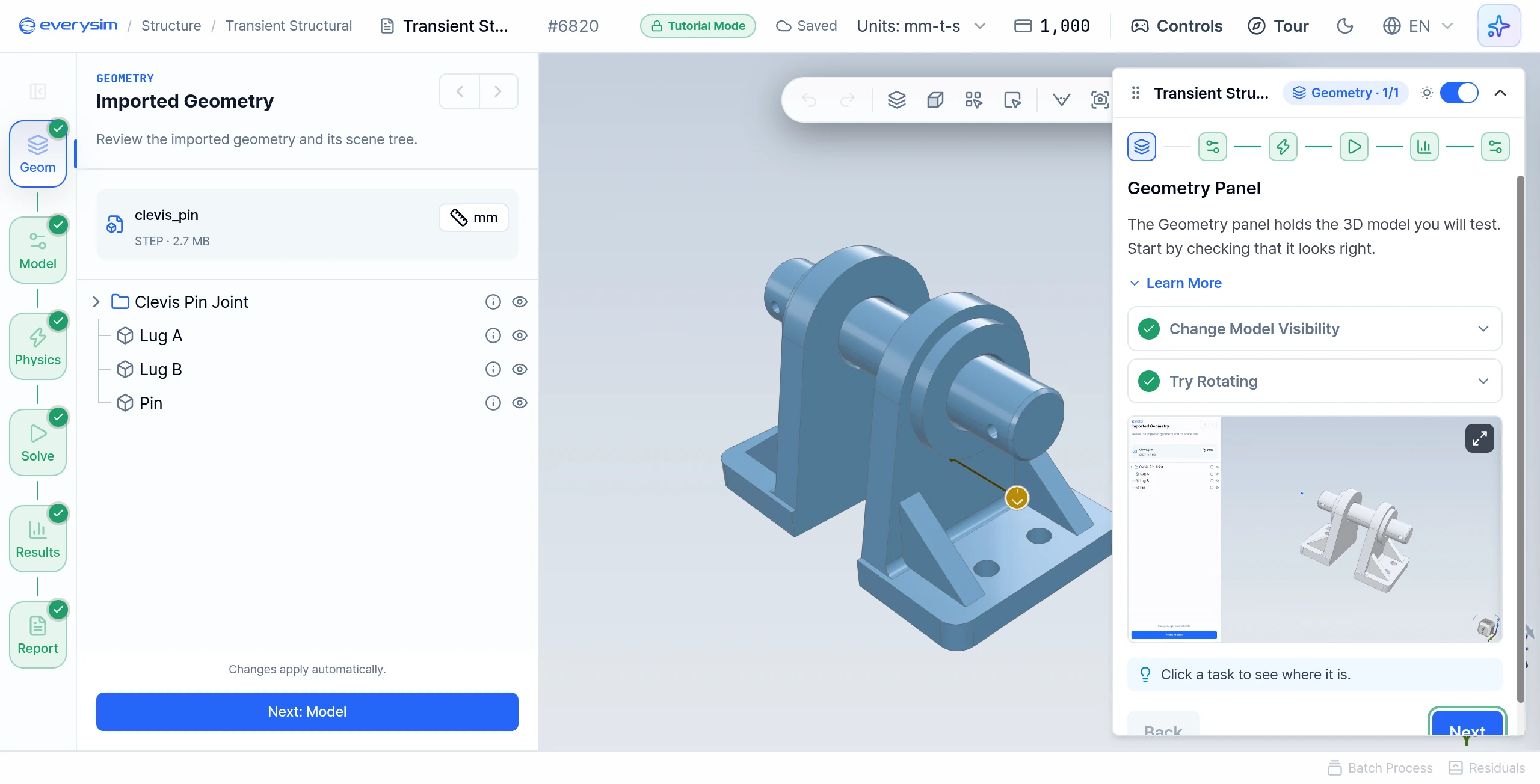
The sample is a clevis: two support blocks and the pin through them. The tree lists them as Lug A, Lug B and Pin under Clevis Pin Joint.
- Change Model Visibility: toggle the eye icon to hide the model, then show it again.
- Try Rotating: drag in the 3D viewport to rotate the model.
2. Material Properties
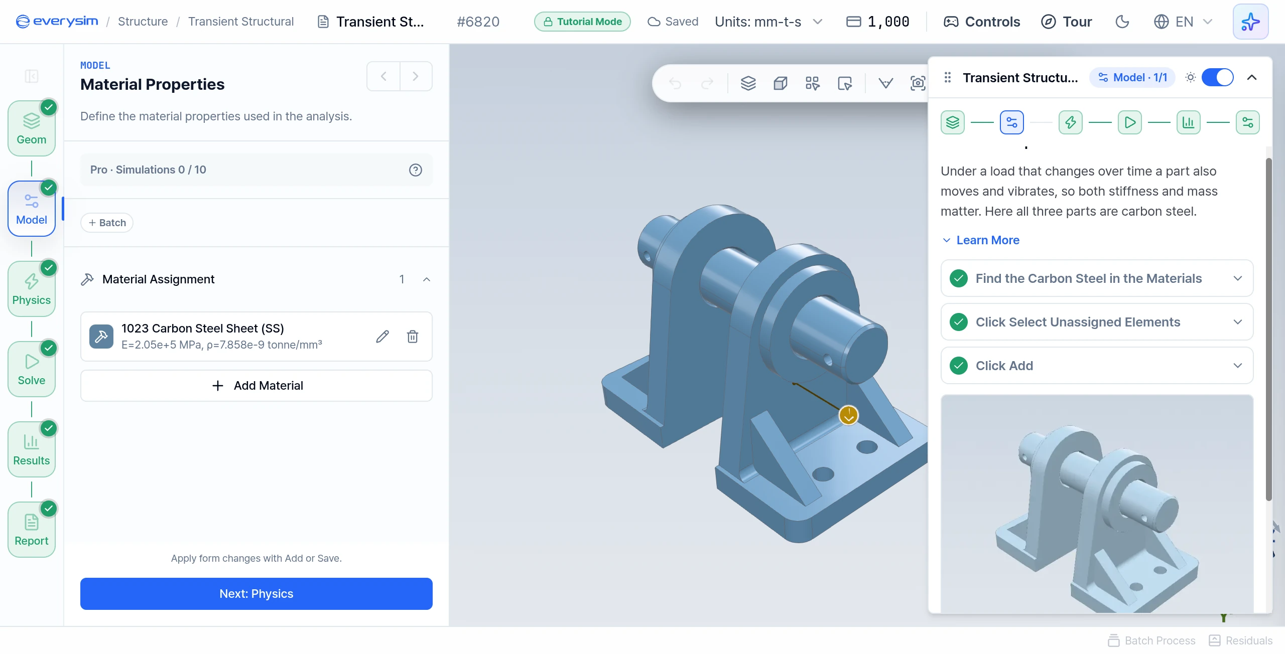
Under a load that changes over time, a part also moves and vibrates. Stiffness controls how much it deforms, and density controls how strongly it resists being set in motion.
- Find the Carbon Steel in the Materials: click Add Material, open Metals and then Steel, and choose 1023 Carbon Steel Sheet (SS). Its yield strength comes with it.
- Click Select Unassigned Elements: the clevis has three parts and only one is picked so far. This picks all of them.
- Click Add: check that all three parts are shown in the material colour, then click Add.
3. Physics Panel
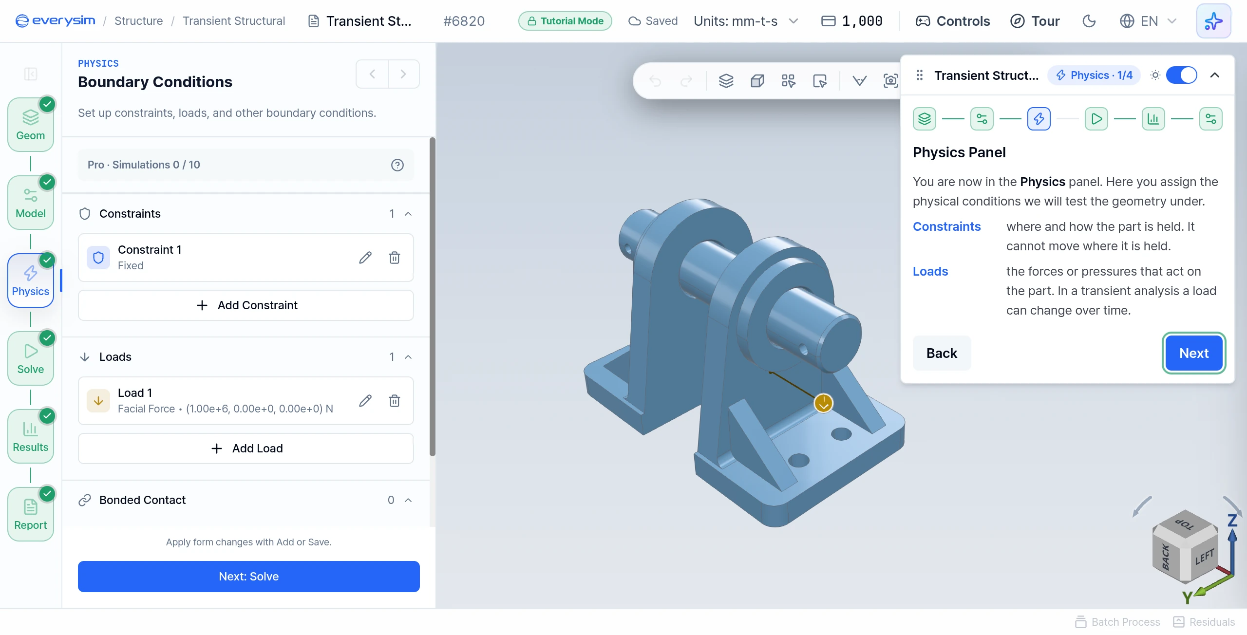
Here you assign the physical conditions. This page has no task.
- Constraints: where and how the part is held. It cannot move where it is held.
- Loads: the forces or pressures that act on the part. In a transient analysis a load can change over time.
4. Constraints
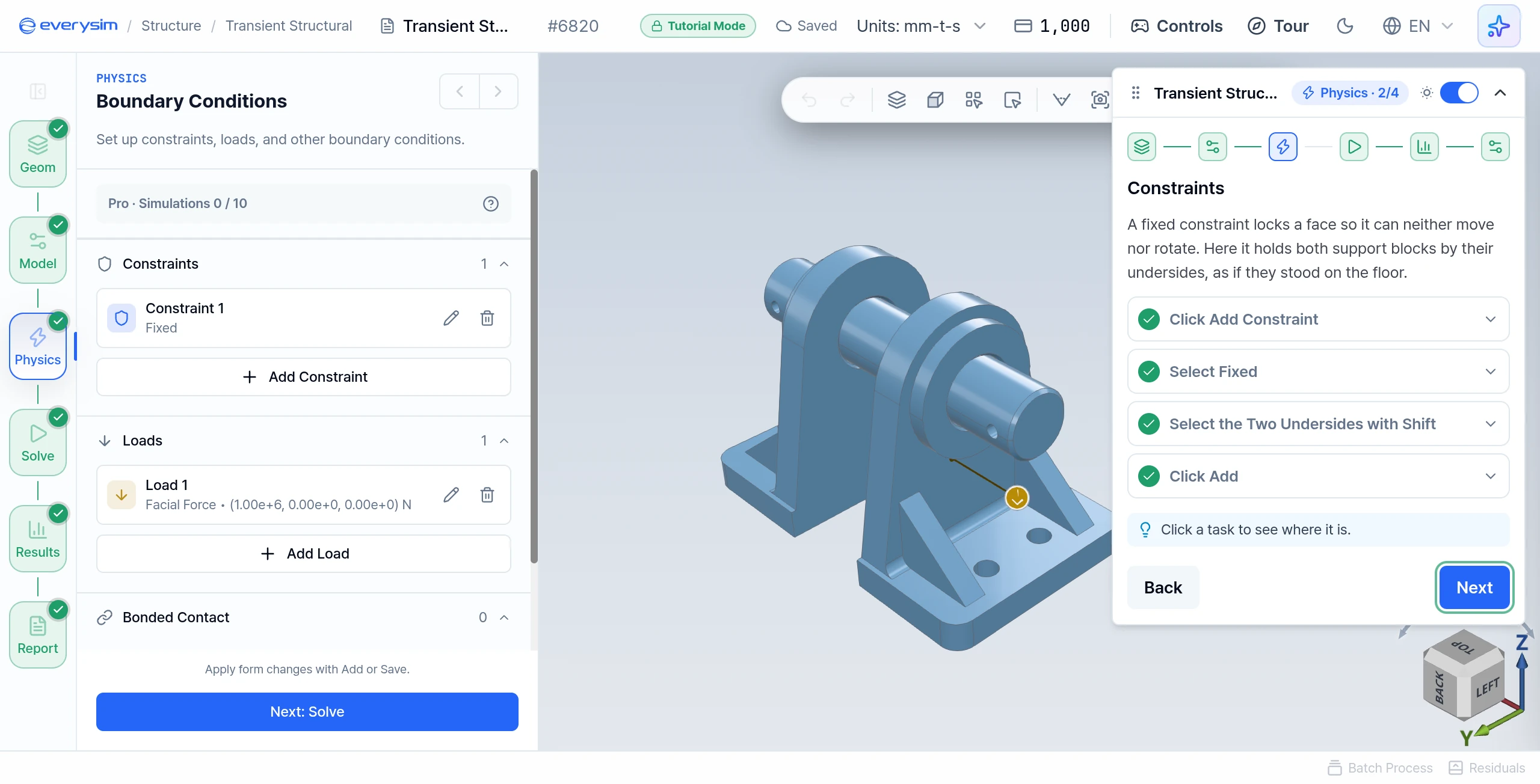
A fixed constraint locks a face so it can neither move nor rotate. Here it holds both support blocks by their undersides, as if they stood on the floor.
- Click Add Constraint in the Constraints section.
- Select Fixed: click Fixed under Type.
- Select the Two Undersides with Shift: the view turns to look at the model from below. Click the underside of one support block, then hold Shift and click the other.
- Click Add to save the constraint.
5. Pulsed Load
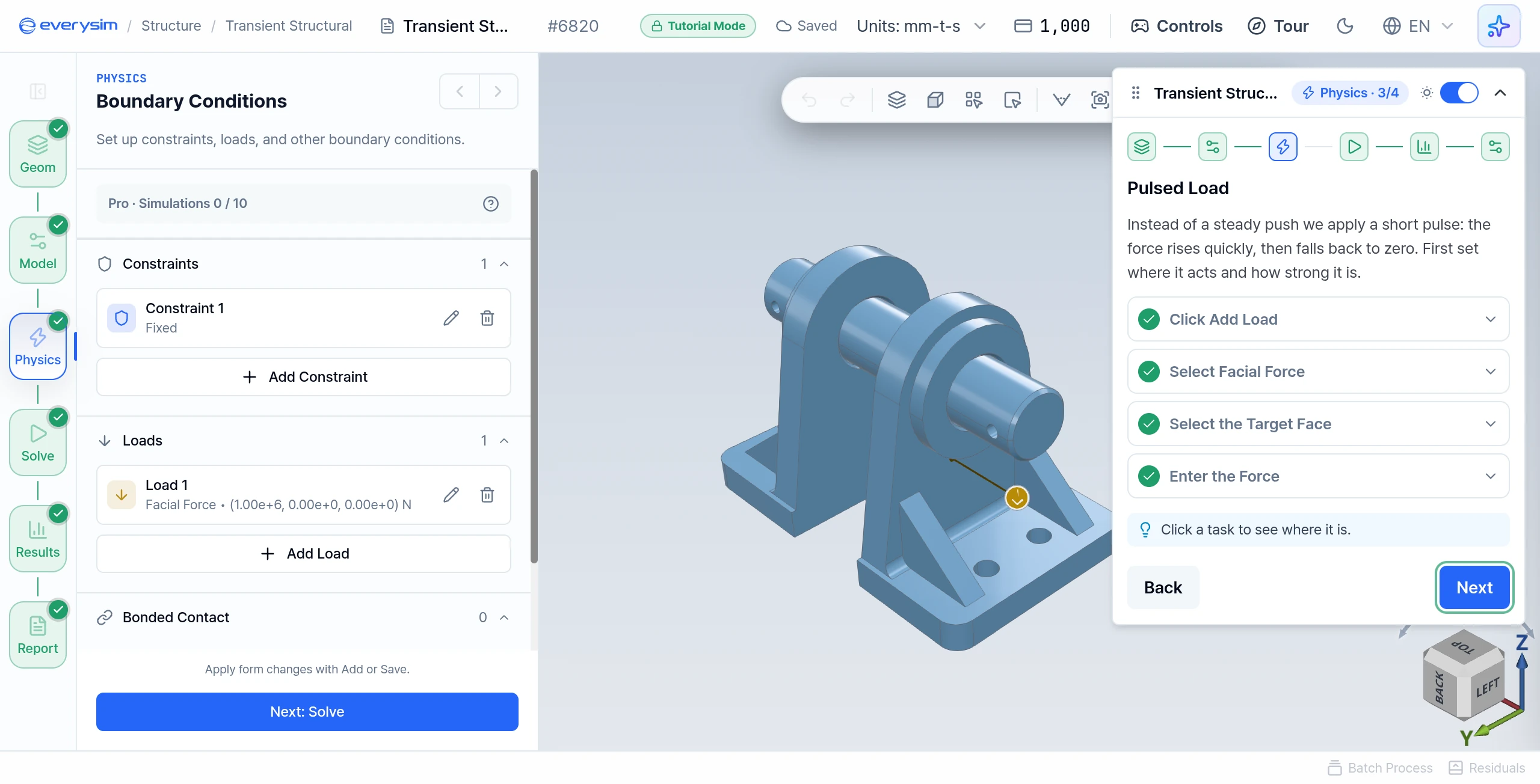
Instead of a steady push, the tutorial applies a short pulse: the force rises quickly, then falls back to zero. First set where it acts and how strong it is.
- Click Add Load in the Loads section.
- Select Facial Force: click Facial Force under Type.
- Select the Target Face: the view turns to face the outer side of the support block to push. Click that large flat face.
- Enter the Force: type
1000000in Fx and press Enter. The field is in N, so this pushes the block toward the other one with 1,000,000 N. Fy and Fz stay0.
6. Pulse Shape
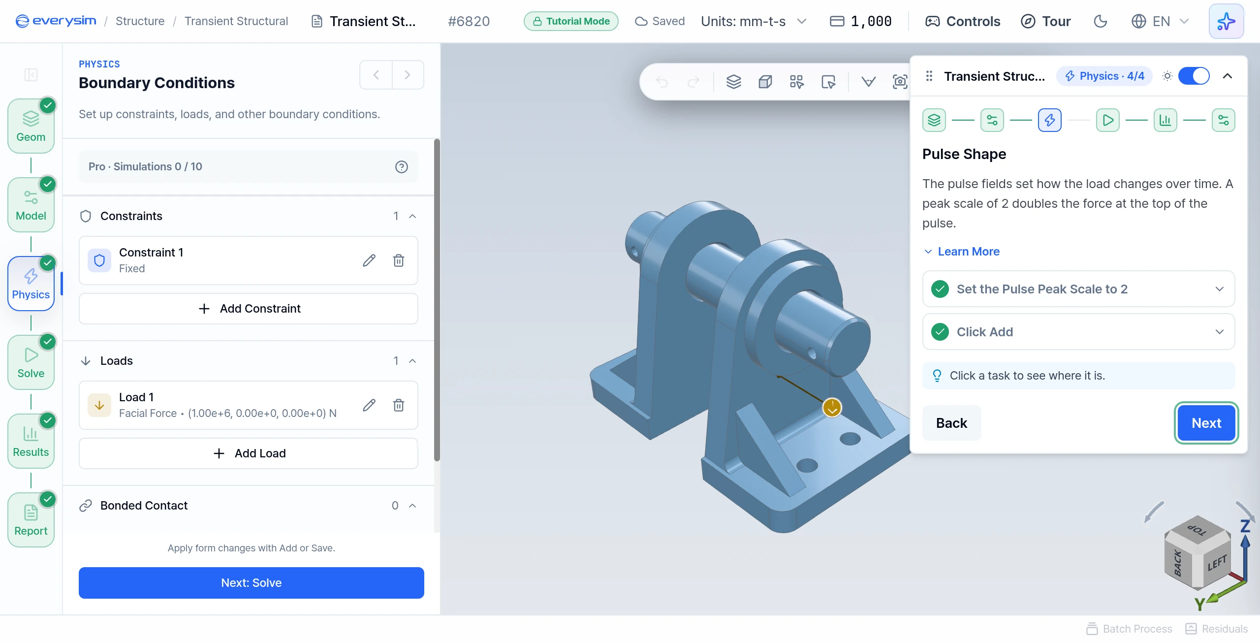
The pulse fields, still in the same load form, set how the load changes over time.
- Pulse Shape: Pulse rises, holds and falls back to zero. Step Load rises and then stays constant to the end of the run. Keep Pulse.
- Pulse Start Time: when the pulse begins.
- Pulse Rise Time, Pulse Hold Time, Pulse Fall Time: how quickly the load ramps up, how long it stays at its peak, and how quickly it ramps back down. A hold time of 0 gives a triangle.
- Pulse Peak Scale: multiplies the magnitude at the top of the pulse.
- Load Profile: draws the result below the fields.
- Set the Pulse Peak Scale to 2: type
2and press Enter. The peak force becomes twice the value you entered. Keep the default rise, hold and fall times. - Click Add to save the load.
7. Transient Parameters
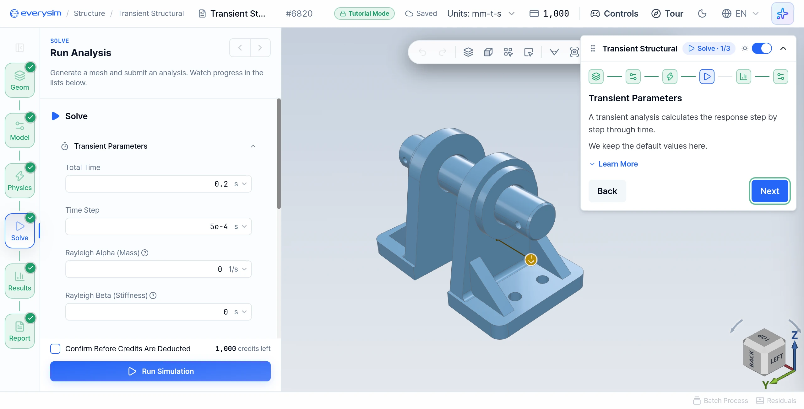
A transient analysis calculates the response step by step through time. This page has no task. Keep the default values:
| Field | Value | Meaning |
|---|---|---|
| Total Time | 0.2 s | How long a period is simulated. |
| Time Step | 5e-4 s | The interval between calculated moments. It must be small enough to capture the pulse. |
| Rayleigh Alpha (Mass) | 0 1/s | Damping, with the value below. |
| Rayleigh Beta (Stiffness) | 0 s | With both at 0, the part keeps vibrating. |
8. Solve Settings
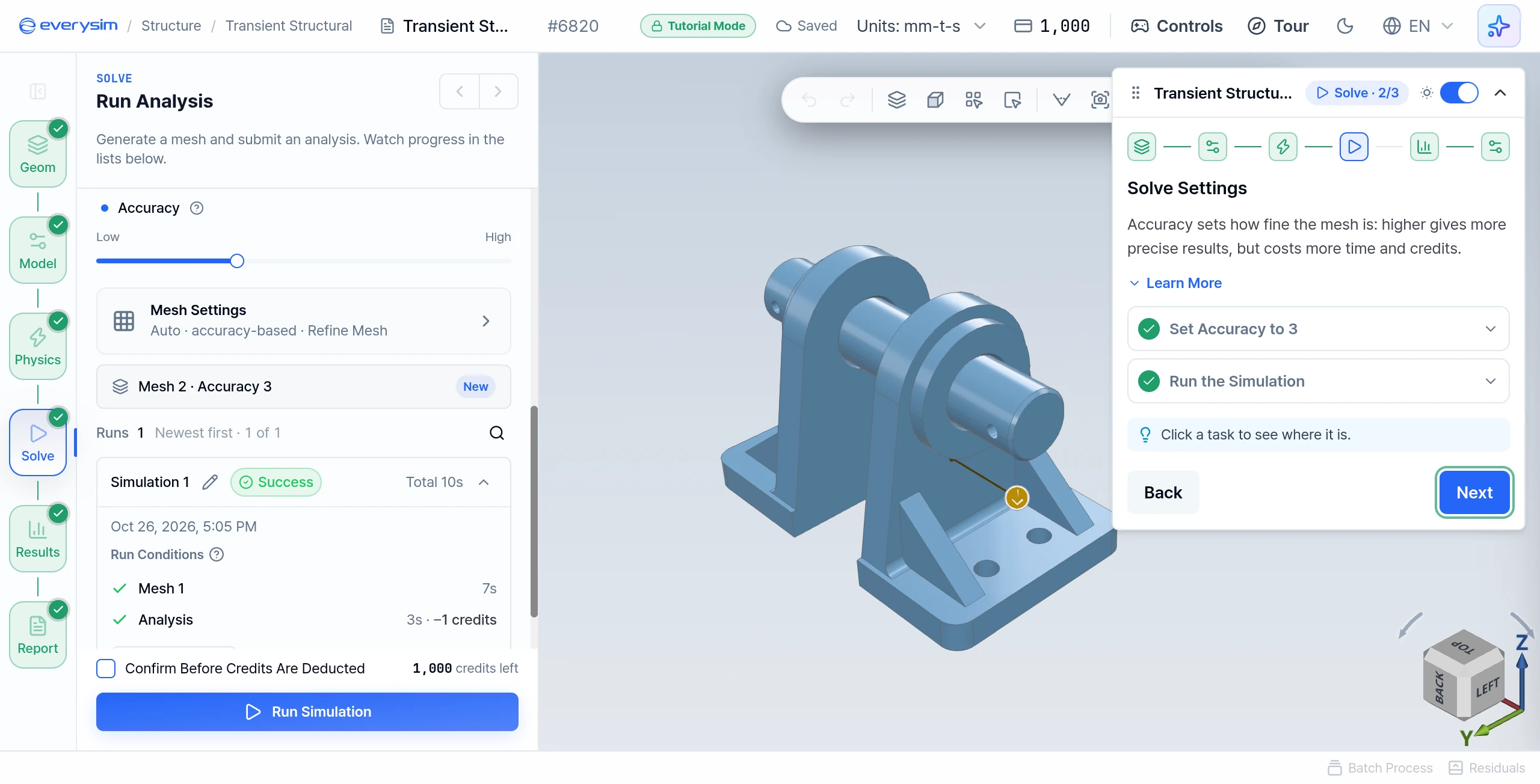
Accuracy sets how fine the mesh is: higher gives more precise results, but costs more time and credits.
- Set Accuracy to 3: move the slider to
3. The project starts lower, so the slider has to move. - Run the Simulation: click Run Simulation at the bottom of the Solve panel.
A tutorial's Run does not submit a job and costs no credits. After about 3 seconds it opens a result computed in advance for this setup. The simulation card can still show an amount such as −1 credits, but tutorial runs are not charged.
9. Simulation Progress
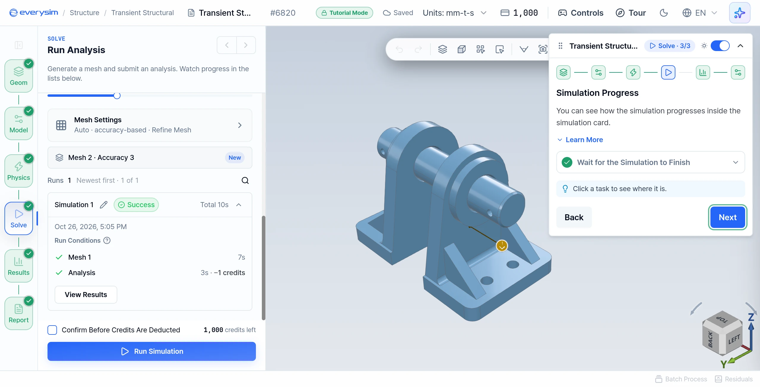
Wait for the Simulation to Finish: the simulation card shows the mesh step and then the analysis steps, each ticked as it completes. When the run is marked Success, the guide moves on and the results open.
10. Your Results
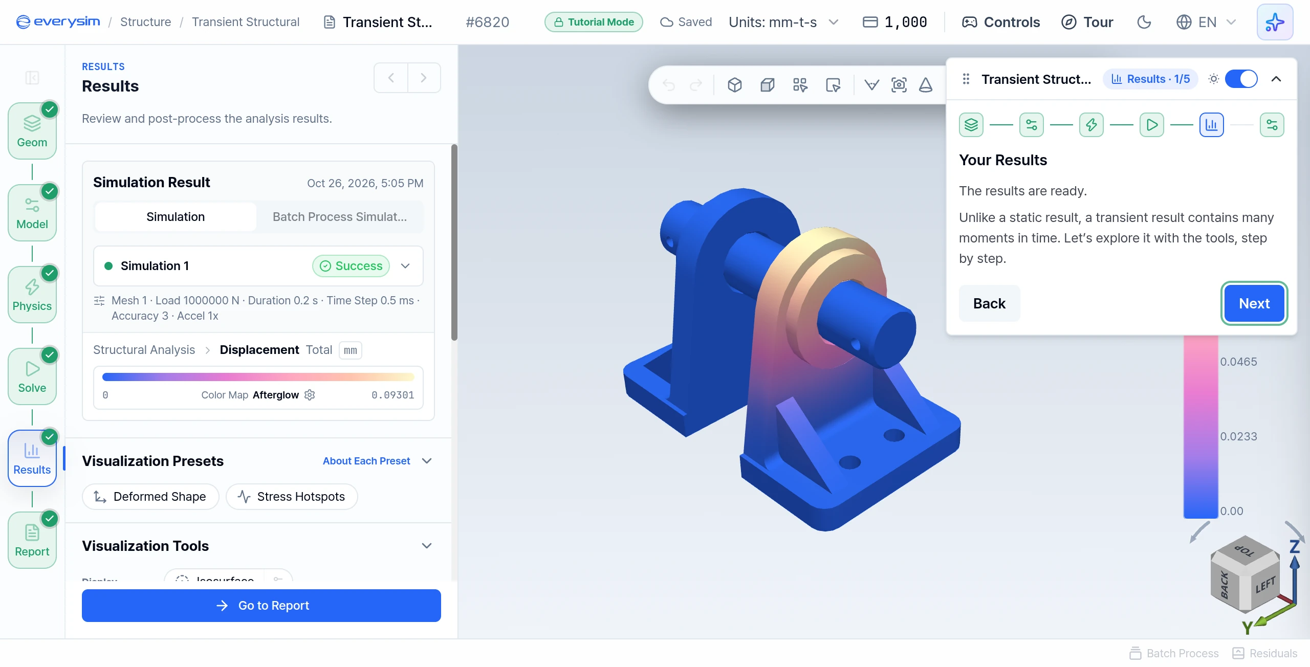
Unlike a static result, a transient result contains many moments in time. Press Next to explore it.
11. Deformation Over Time
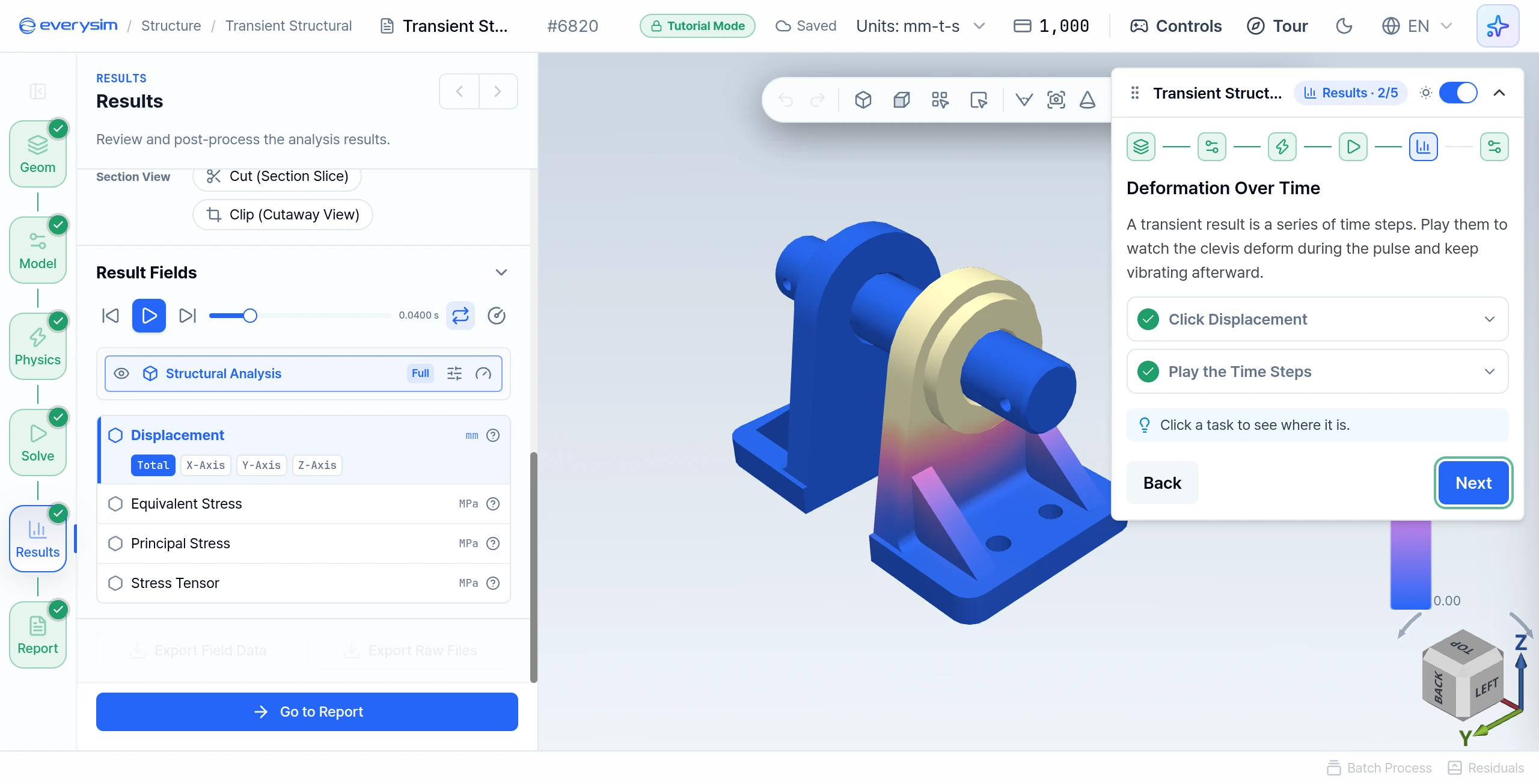
A transient result is a series of time steps. Play them to watch the clevis deform during the pulse and keep vibrating afterward.
- Click Displacement in the result fields.
- Play the Time Steps: press Play beside the slider in Result Fields.
12. Stress Over Time
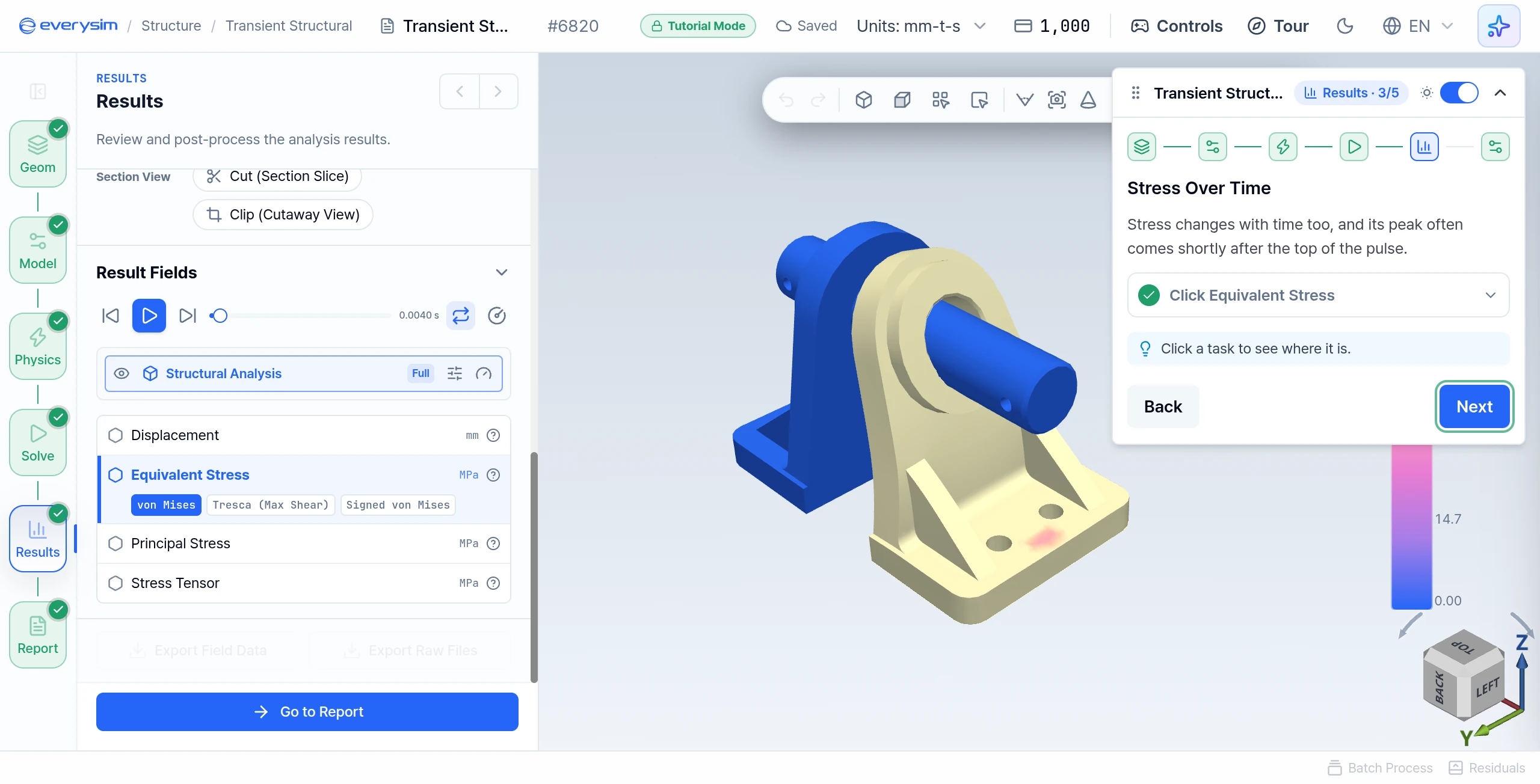
Stress changes with time too, and its peak often comes shortly after the top of the pulse.
- Click Equivalent Stress in the result fields. It opens on von Mises, so you see how the stress is spread.
The figure has the slider at 0.004 s, the frame where this result peaks. The slider moves in frames 0.004 s apart.
13. Change the Color Map
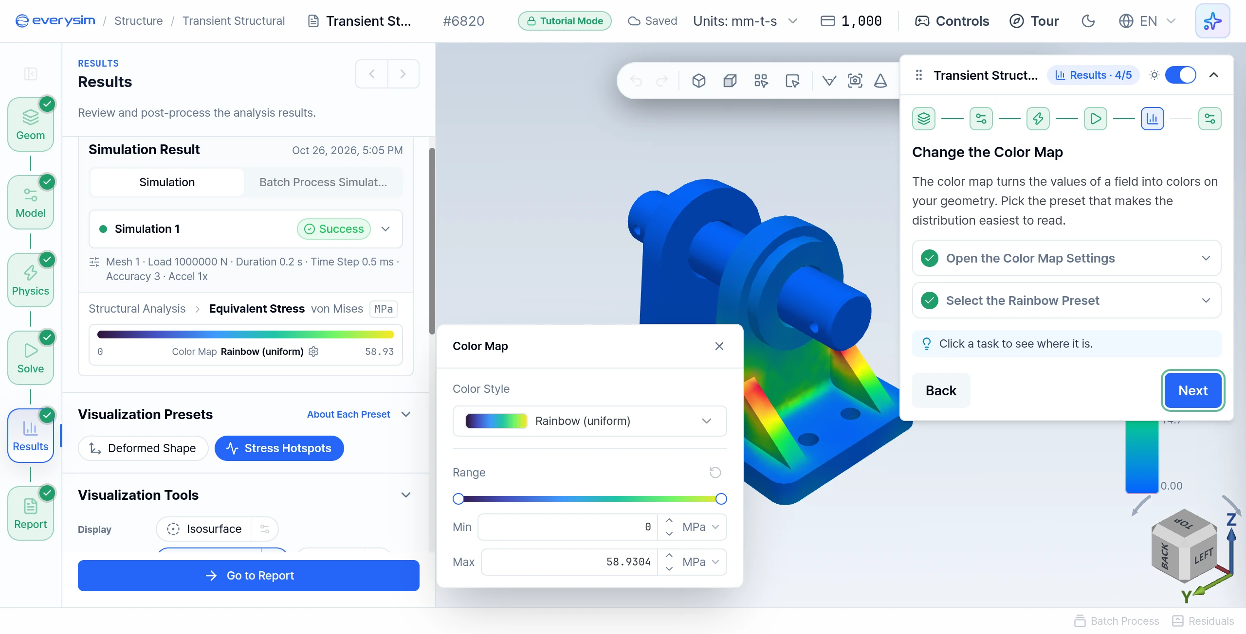
The color map turns the values of a field into colors on the geometry.
- Open the Color Map Settings: click the color map bar in the Simulation Result card.
- Select the Rainbow Preset: choose Rainbow (uniform) under Color Style.
14. Report
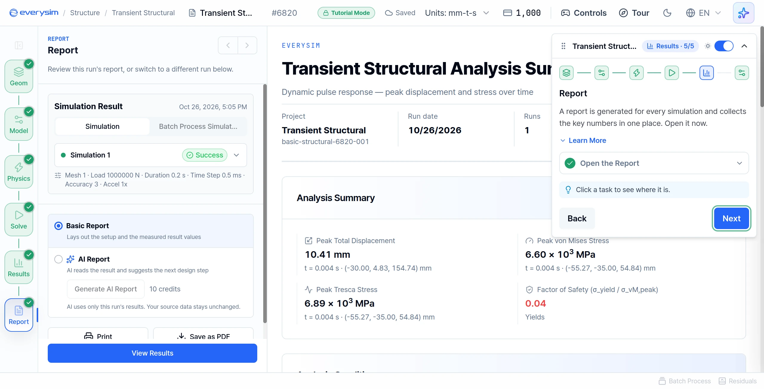
A report is generated for every simulation and collects the key numbers in one place.
- Open the Report: click Go to Report at the bottom of the panel. The guide moves on by itself.
15. Core Results
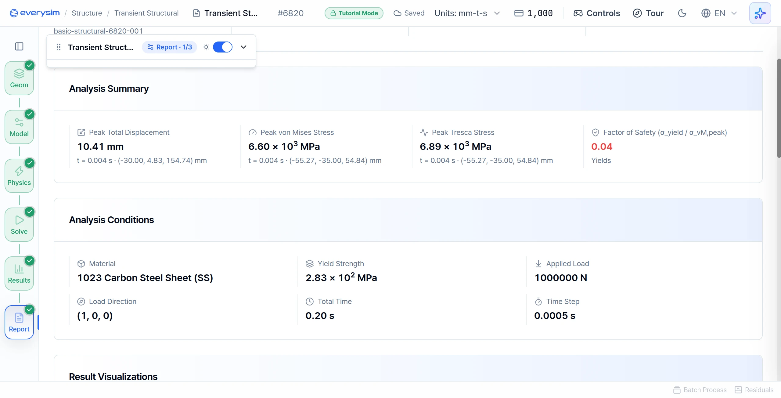
For a transient analysis the report lists peak values: the highest value reached at any moment of the run. The prepared result reads:
| Report item | Value |
|---|---|
| Peak Total Displacement | 10.41 mm at t = 0.004 s |
| Peak von Mises Stress | 6.60 × 10³ MPa at t = 0.004 s |
| Peak Tresca Stress | 6.89 × 10³ MPa at t = 0.004 s |
| Factor of Safety (σ_yield / σ_vM,peak) | 0.04, Yields |
| Material | 1023 Carbon Steel Sheet (SS) |
| Yield Strength | 2.83 × 10² MPa |
| Applied Load | 1000000 N |
| Load Direction | (1, 0, 0) |
| Total Time | 0.20 s |
| Time Step | 0.0005 s |
The factor of safety compares the yield strength with the peak stress:
Below 1, the part yields at some moment during the pulse. Here it is far below 1, so the report reads Yields.
16. Stress History
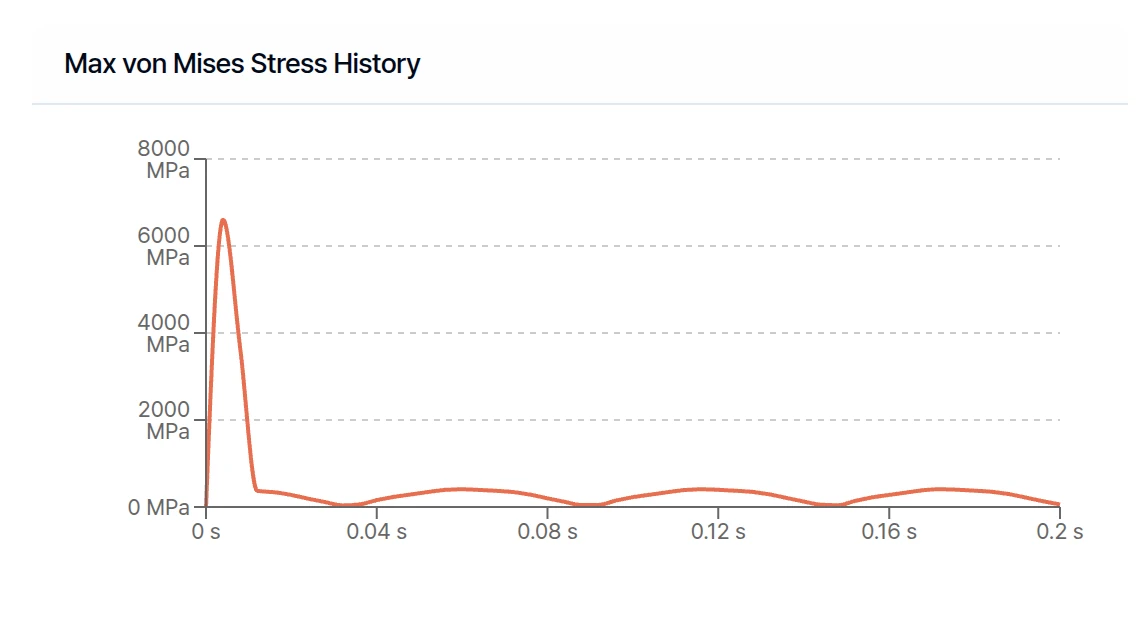
Max von Mises Stress History shows the highest von Mises stress at each time step. The top of the curve is the peak value from the table. Nothing damps the vibration, so the curve keeps oscillating after the pulse ends.
17. Displacement History
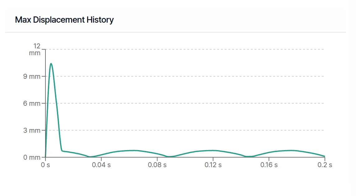
Max Displacement History shows the highest displacement at each time step. Compare it with the stress curve. If the two rise and fall together, the stress comes directly from how far the part is deformed.
Press Finish on this page to complete the tutorial. You now know how to set up a load that changes over time and read how the structure responds.
Need Assistance or Have Questions?
Frequently Asked Questions: FAQ Link
Support Inquiries: support@everysim.io