4.5 Fluid Dynamics: Component-Wing
1. Geometry
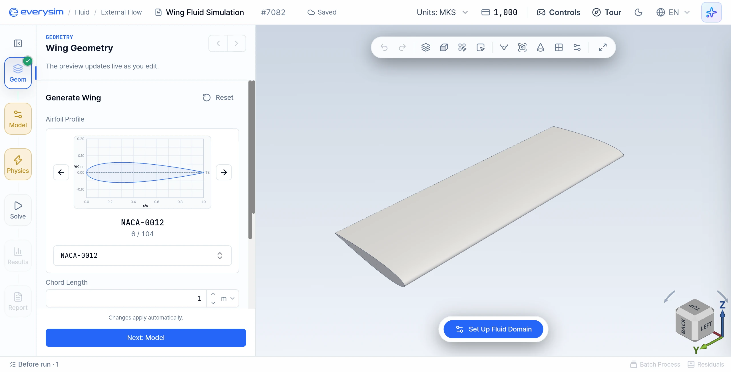
This screen shows the wing creation step for fluid dynamics analysis. The user selects an airfoil from the searchable airfoil list, checks the airfoil preview, and enters the wing settings. The left rail shows the workflow: Geom (Geometry), Model, Physics, Solve, Results, Report.
At the first step, create the wing geometry that will be used for fluid dynamics analysis.
1.1. Parametric Design
In the parametric wing creation interface, you can generate a wing by selecting an airfoil and defining basic geometric settings.
The main configuration items are:
- Airfoil Profile: Search and select the airfoil profile to use for the wing section
- Chord Length: Defines the chord length of the wing section
- Span: Defines the span of the wing
- Spline: Controls the spline interpolation of the airfoil curve: none, or 1 to 10
Valid changes generate the wing automatically. When the preview looks right, click Next: Model.
1.2. Reference Dimensions
Check Characteristic Length, typically the chord. It feeds the Reynolds number and the coefficients.
2. Model: Fluid Domain
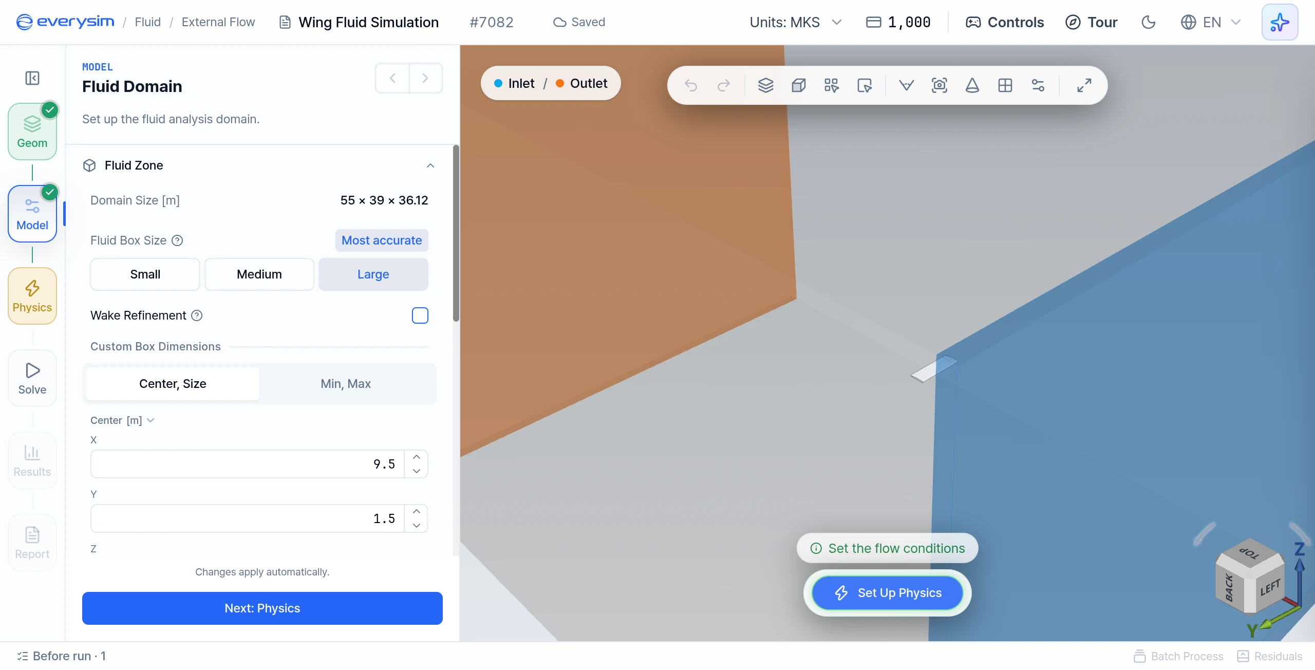
This figure shows the fluid domain panel. The wing sits between the inlet and outlet faces of the fluid domain, which represents the air volume used for aerodynamic analysis.
Opening Model creates the fluid domain automatically. Adjust it if needed and verify that the wing is inside it.
2.1. Fluid Box Size
Choose Small (fastest, for comparing designs), Medium (the standard choice) or Large (slowest, for final numbers). Turn on Wake Refinement to refine the mesh in the wake behind the wing. Drag is more accurate, but the run takes longer.
2.2. Custom Box Dimensions
For exact values, use Custom Box Dimensions with the Center, Size or Min, Max tab.
- Center: X, Y and Z position of the center of the domain
- Size: Length of the domain in the X, Y and Z directions
If the box is too tight for the wing, the app shows a warning.
2.3. Fluid Properties
Choose Air, Water or Custom. This changes the coefficients and the Reynolds number.
3. Physics: Flow Conditions
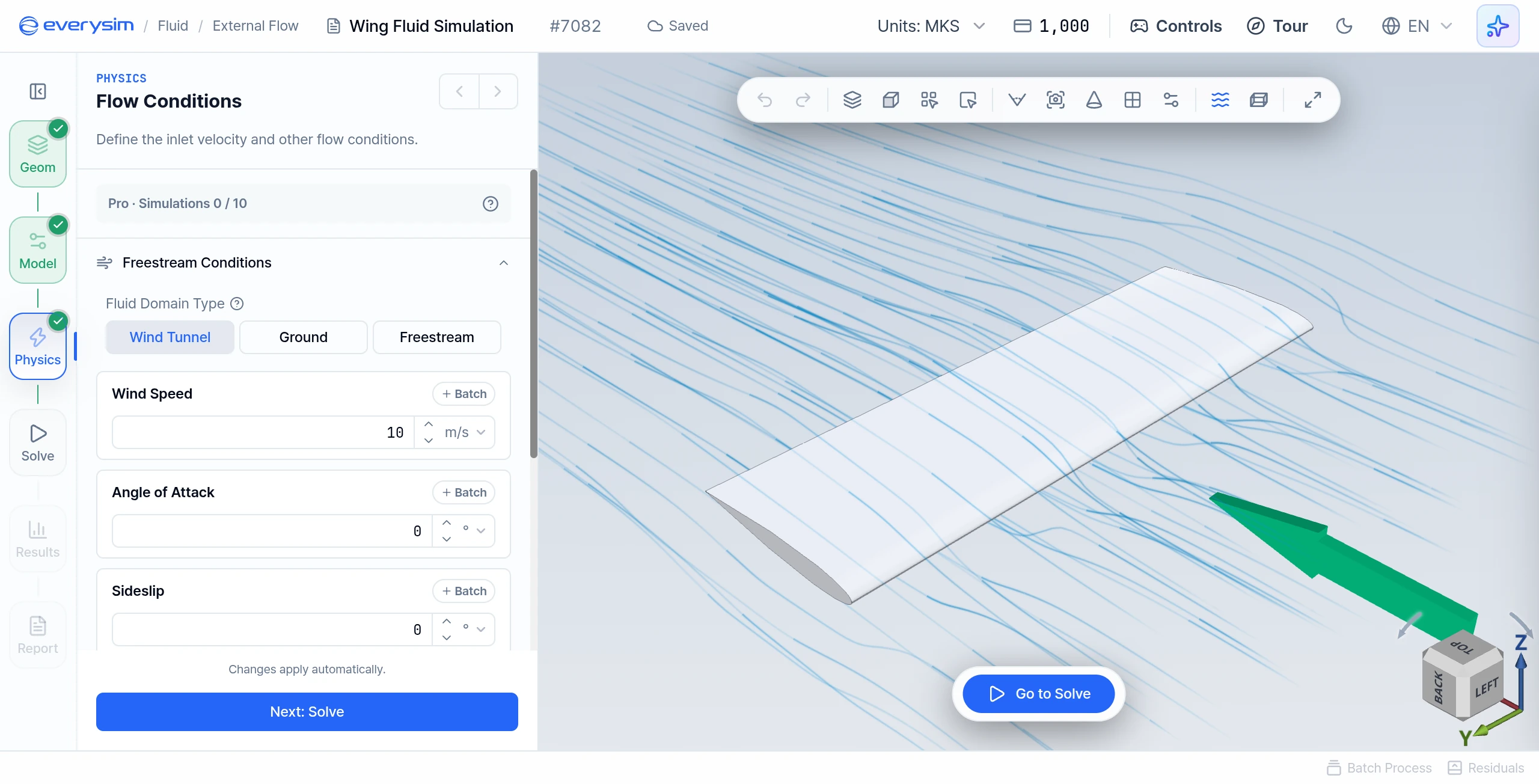
This screen shows the Flow Conditions panel after the wing and fluid domain have been created. Configure the incoming flow here before running the analysis.
- Fluid Domain Type: Wind Tunnel, Ground or Freestream
- Wind Speed: Defines the inflow velocity applied to the fluid domain
- Angle of Attack and Sideslip: Set the attitude of the wing relative to the flow
- Flow Direction: The direction the wind travels, from inlet to outlet. Auto is the default.
- Lift Direction: The direction of lift. Auto is the default.
4. Solve
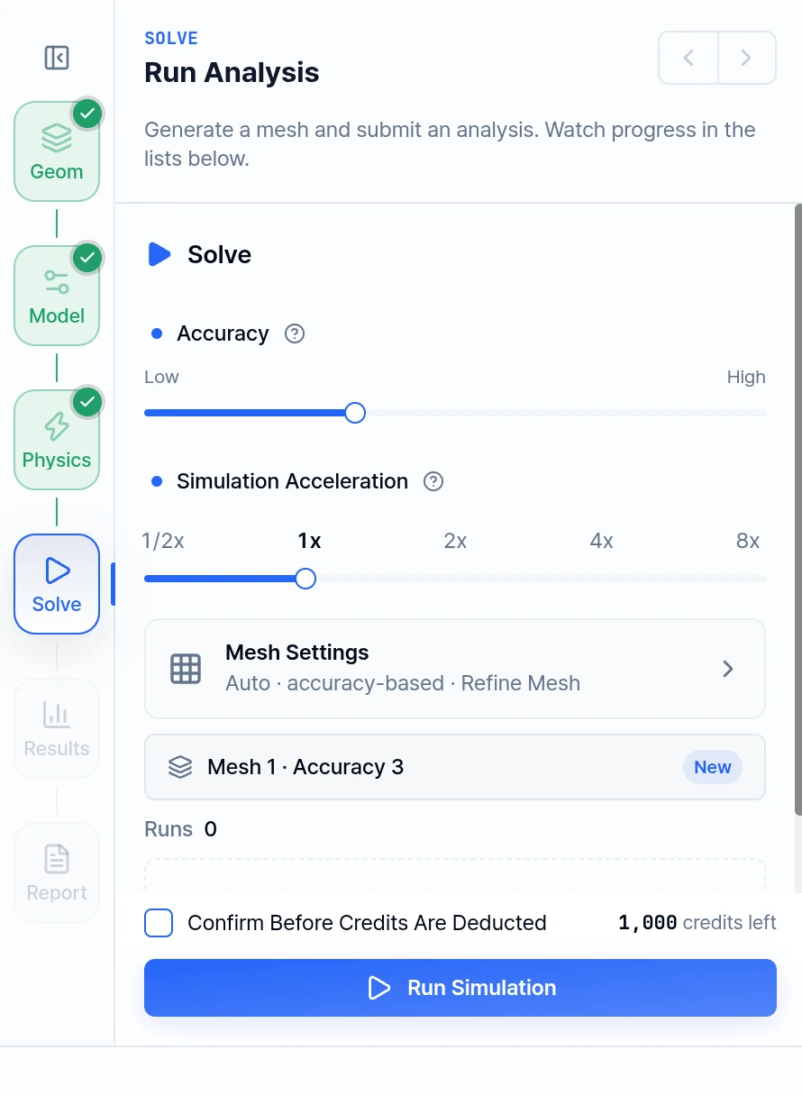
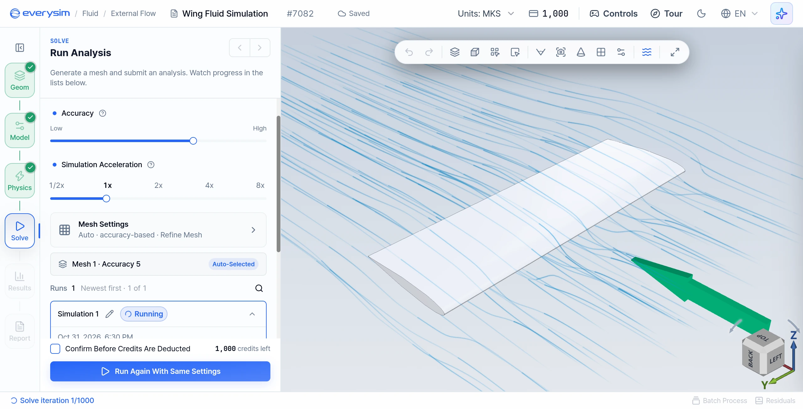
This figure shows the Solve step during a run. The 3D viewer displays the meshed fluid domain around the wing, and the panel holds the mesh and run settings.
- Accuracy: A 7-step slider from Low to High. Higher accuracy gives more precise results, but takes longer and uses more credits.
- Mesh Settings: With Auto Size on, sizes follow Accuracy. With it off, the slider has no effect and you set Mesh Detail, Size Transition Smoothness, Shape Accuracy, Edge Refinement and Shape Accuracy Method (Standard, Adaptive, Precise, Maximum Precision). The toggles are Refine Mesh, Feature Smoothing and Detail Capture (Beta).
- Simulation Acceleration: 1/2x to 8x. Higher acceleration shortens the run and consumes credits faster; stops above your plan limit are locked.
- Run Simulation: Generates the mesh if needed, then starts the solve.
- Generate Mesh Only: Generates the mesh so you can preview it first.
Before running the simulation, confirm that the Geometry, Model, and Physics steps are complete.
5. Residuals
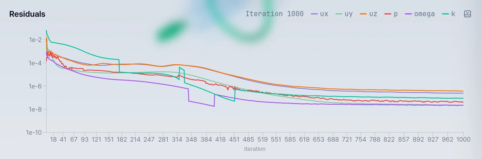
This screen shows the residual graph generated during the CFD simulation. Each curve represents the numerical residual of a simulation variable over the iteration history. By observing whether the curves decrease and stabilize, the user can evaluate whether the flow solution is converging properly.
When solving starts, the Residuals chart opens at the bottom of the workbench. Residual curves are used to check whether the numerical solution is stabilizing during the calculation.
Use the residual plot to:
- Track the progress of each solution variable
- Check whether the simulation is converging
- Identify unstable or oscillating behavior during the run
After the simulation is complete, review the aerodynamic results generated from the analysis.
6. Results
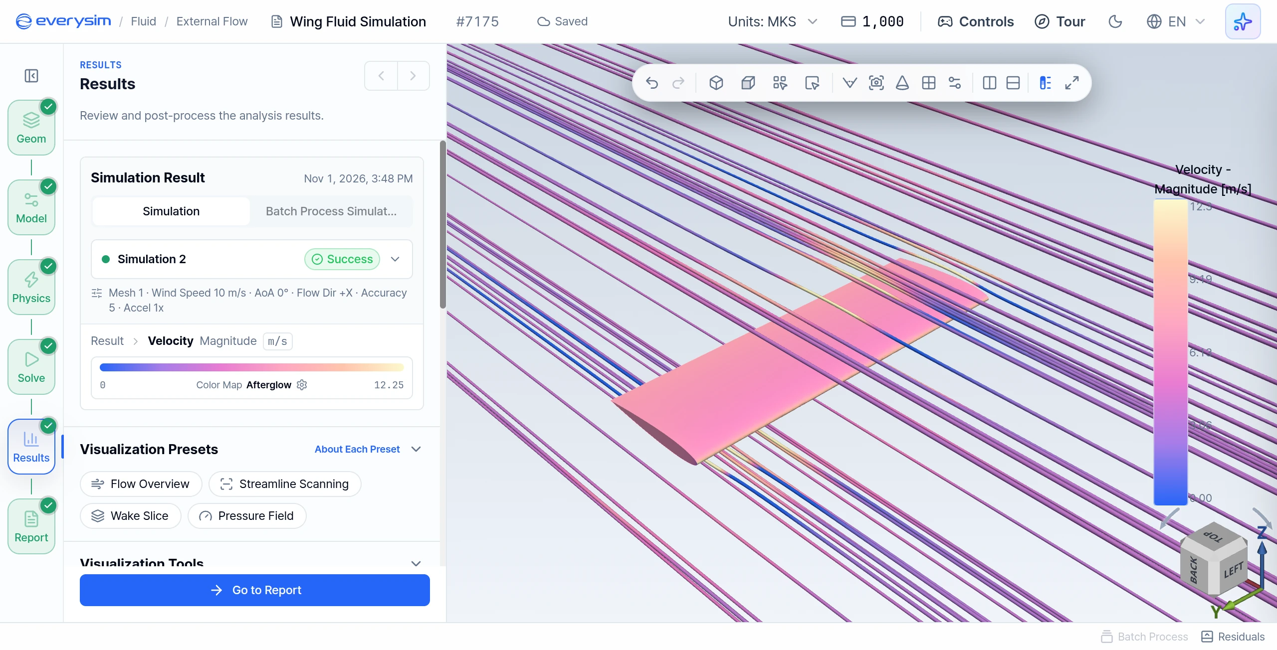
Figures 7 to 9 are from a NACA-0012 wing at 10 m/s and 0° angle of attack in a Wind Tunnel domain, at Accuracy 5. In Figure 7 the fluid domain is hidden by setting the Opacity of Result to 0 under Result Fields, with Streamline on.
The Results stage provides volume and body-surface fields including velocity, pressure, turbulence quantities, advanced vorticity, vorticity, and wall shear stress. Select a result field in the Results Tree, then use the legend and viewer tools to interpret its range.
Turn on Streamline under Visualization Tools to seed flow lines. Adjust Position, Lines, Thickness and Max Length to reveal flow direction and wake behavior without obscuring the wing. Compare surface pressure with the surrounding velocity field before drawing conclusions about lift or separation.
7. Report
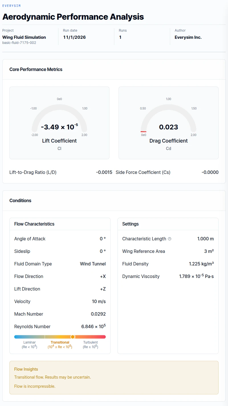
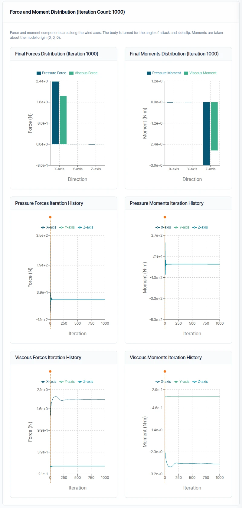
The NACA-0012 section is symmetric, so at 0° angle of attack the lift is effectively zero: Lift Coefficient -3.49 × 10⁻⁵, Drag Coefficient 0.023.
The report summarizes lift and drag coefficients, freestream velocity, Mach number, Reynolds number, reference dimensions, fluid properties, and the force-and-moment history. Flow insights identify the calculated regime and whether the incompressible-flow assumption is being used.
When comparing wing variants, keep the reference area, characteristic length, flow speed, angle of attack, sideslip, domain size, accuracy, and fluid properties consistent.
Need Assistance or Have Questions?
Frequently Asked Questions: FAQ Link
Support Inquiries: support@everysim.io