4.6 Fluid Dynamics: Simulation on Your CAD
This page runs a fluid simulation on your own CAD model, from upload through the report. Use it for any body the propeller and wing pages do not generate for you: a full aircraft, a fuselage, a vehicle, or a general 3D shape.
To start, go to New Project and choose either path. Both open the same workflow:
- Fluid Dynamics (CFD) > External Flow > Stationary Body
- EveryDrone > Fluid Dynamics > Integration Testing
There is no separate Aircraft or Custom option. Projects created with either older option open in this workflow.
1. Upload CAD
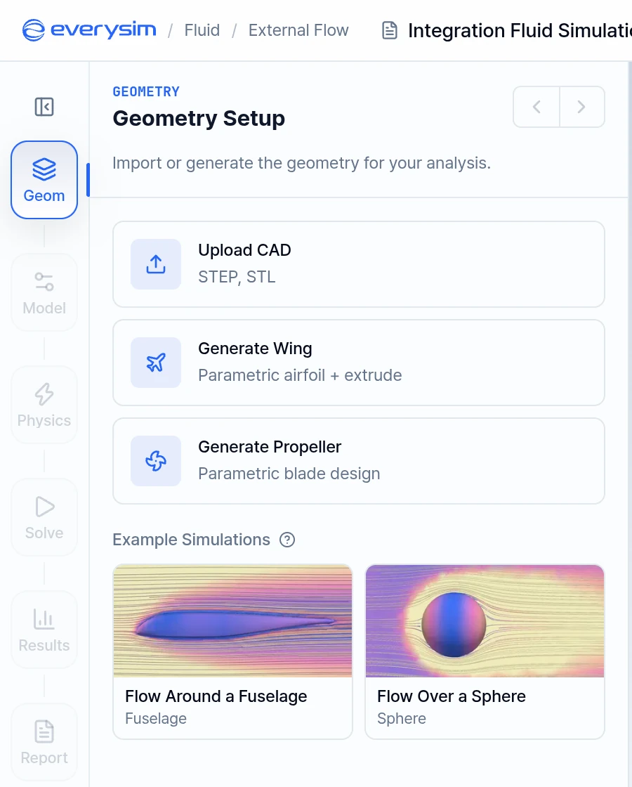
The Geometry step opens on Geometry Setup. Choose Upload CAD. Generate Wing and Generate Propeller build a parametric model instead.
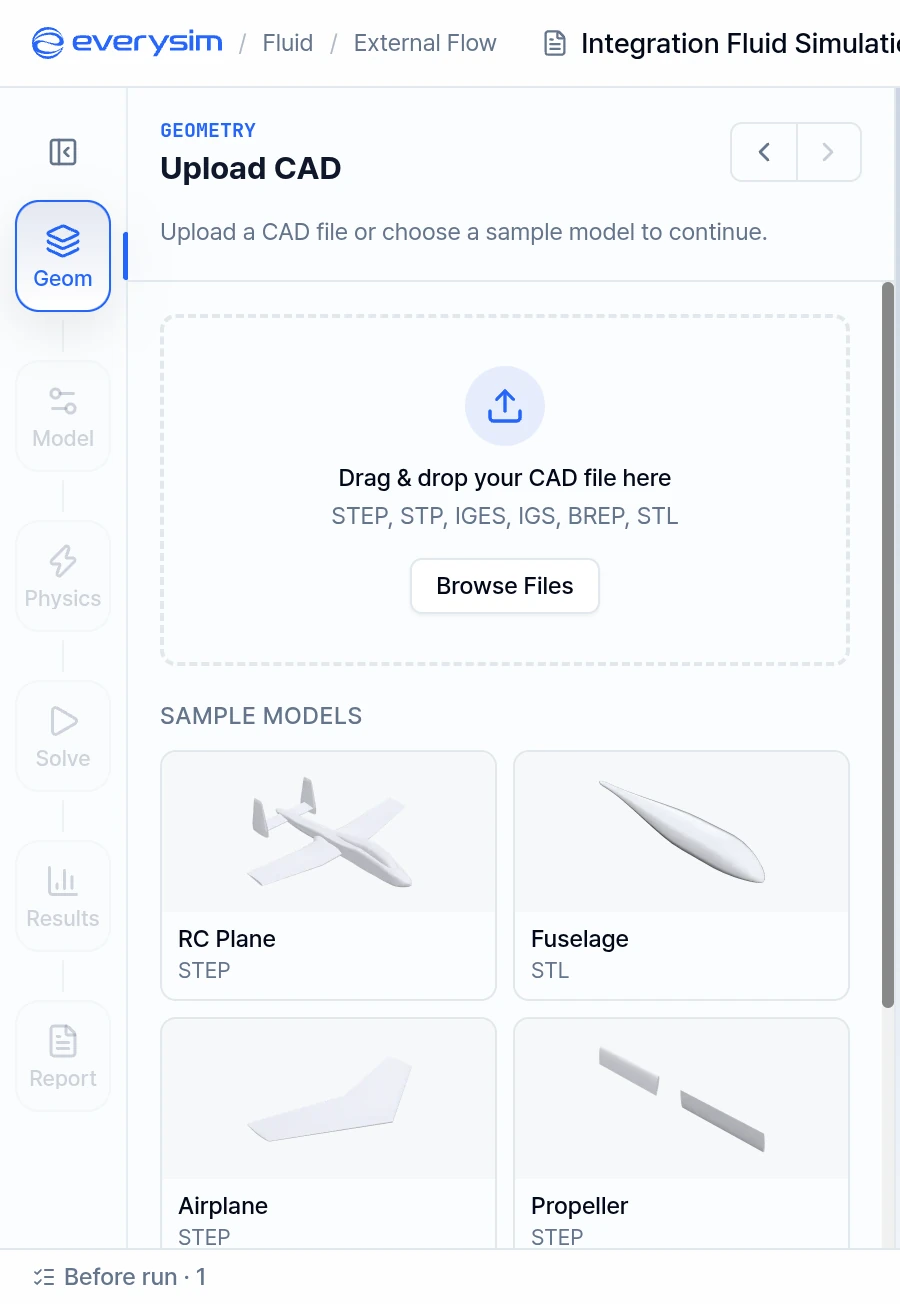
Drag a file onto the upload area or click Browse Files. Selecting a file starts the import.
- Supported formats: STEP, STP, IGES, IGS, BREP and STL. The Upload CAD card in Figure 1 names only STEP and STL, but all six are accepted.
- Sample Models: To try the workflow without your own file, choose RC Plane, Fuselage, Airplane, Propeller, Rocket or Car.
- Example Simulations: On Geometry Setup, Flow Around a Fuselage and Flow Over a Sphere load a geometry with preset settings and go straight to Solve.
- Units: Confirm the length unit if the app asks. An STL file has no unit of its own. A STEP file uses the unit it declares, so change that only if the geometry looks the wrong size.
After the import, check in the viewport that the model has the expected shape and size.
2. Geometry Health
The app inspects your CAD during the import and reports the result on the Geometry step. Simulation geometry needs clean, closed solids with properly connected faces and edges, because defects can prevent reliable meshing.
When it finds a problem, the panel lists the affected parts under Needs Attention, split into Blocking Defects and Warnings. Typical defects include Free Edge, Unclosed Solid and Non-Manifold Edges.
- Blocking Defects: Resolve these before running.
- Warnings: These may affect result accuracy.
- Heal Geometry: Repairs what it can. Fixing one defect can expose another it was masking, so the count may not reach zero in a single pass. Run it again for the remainder.
If the same defects persist, or automatic healing cannot repair them, correct the part in your CAD system and import it again.
For an STL file, issues appear as Risk items such as Hole (Open Edge). Meshing or the simulation may fail on them. If it does, fix the geometry in CAD and export the STL again.
3. Reference Dimensions
Before leaving the Geometry step, set Reference Dimensions. These values define the coefficients in your report.
- Object Type: Sets the area that the lift and drag coefficients use.
- Wing: The planform area.
- Aircraft: The Wing Reference Area you enter. This value is required to run.
- Other: The frontal area. You can enter a Custom Reference Area instead.
- Characteristic Length: A representative distance over which flow develops around the body, such as wing chord, fuselage length, or diameter. It is used for Reynolds number and reference coefficients. For an aircraft, this is typically the Mean Aerodynamic Chord (MAC).
Mean Aerodynamic Chord (MAC):
A reference length used in aerodynamics, particularly for defining characteristics of an aircraft wing.
Click Next: Model to continue.
4. Model: Fluid Domain
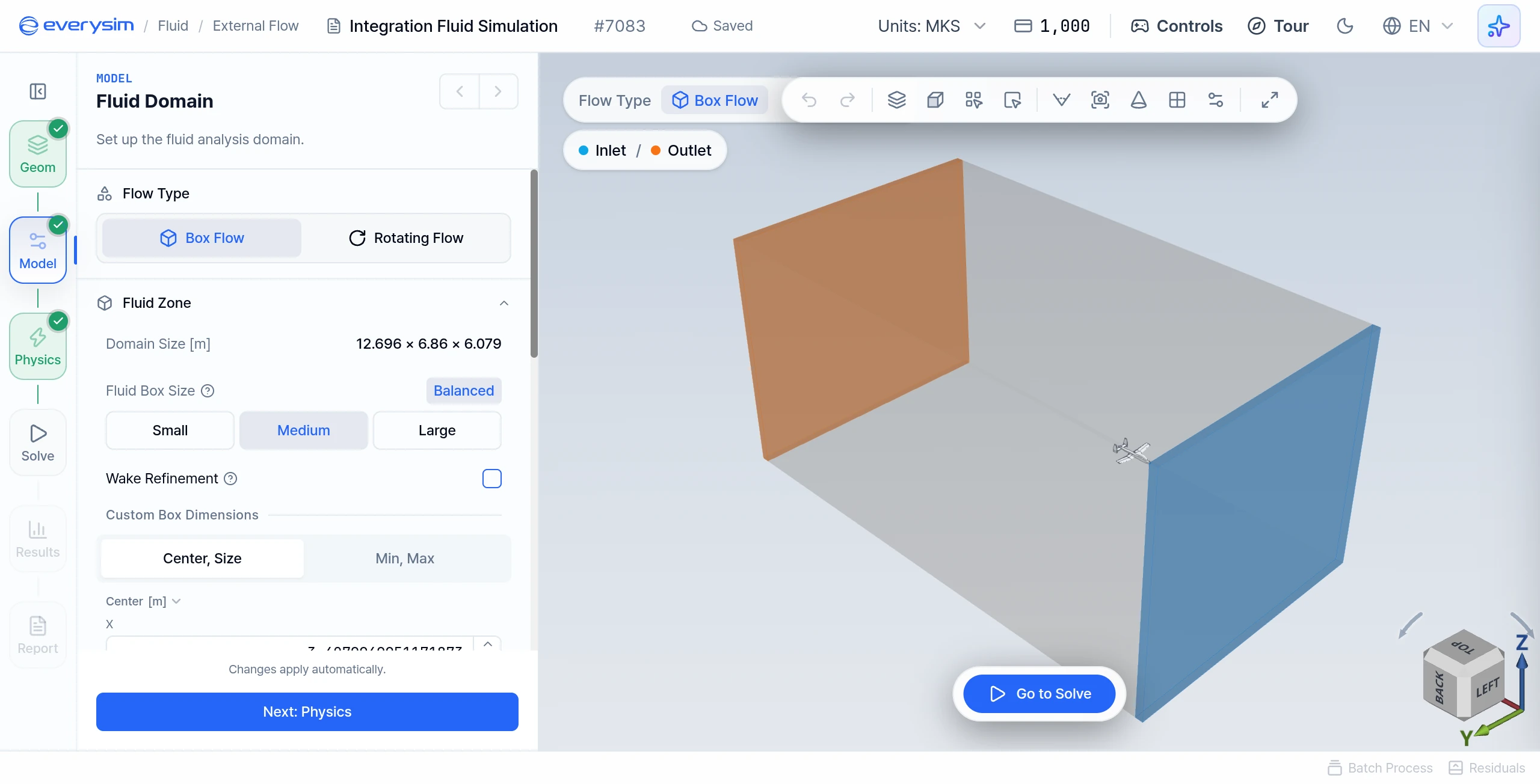
Opening Model creates the domain around your geometry. Adjust it here, then verify that the body sits fully inside the box.
- Flow Type: Box Flow or Rotating Flow. Each type keeps its own settings, and the app asks you to confirm a switch. Rotating Flow uses the zone settings described on the propeller page.
- Fluid Box Size: Small (fastest, for comparing designs), Medium (the standard choice) or Large (slowest, for final numbers).
- Wake Refinement: Refines the mesh in the wake behind the body. Drag is more accurate on bodies with a large wake, but the run takes longer.
- Custom Box Dimensions: Enter exact values on the Center, Size or Min, Max tab. If the box is too tight for the body, the app warns you, because a tight box squeezes the flow and overstates the forces.
- Fluid Properties: Choose Air, Water or Custom. This changes the coefficients and the Reynolds number.
5. Physics: Flow Conditions
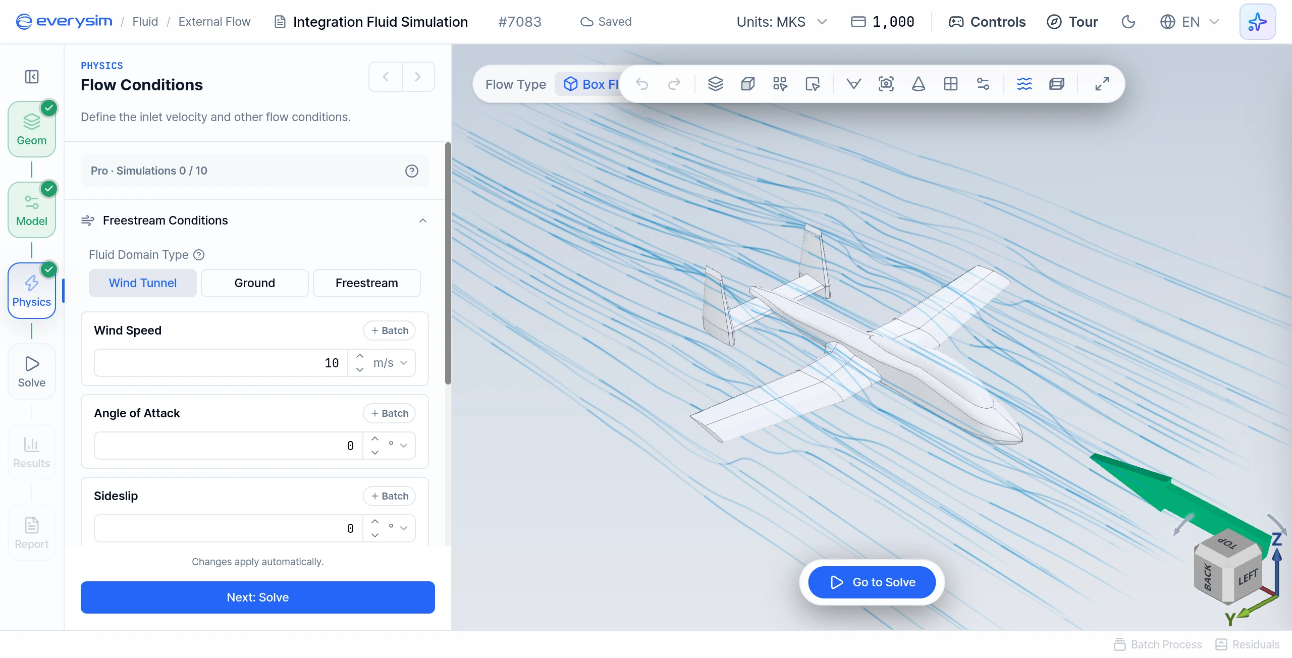
The Physics step defines the incoming flow.
- Fluid Domain Type: Wind Tunnel (solid walls around the model), Ground (a floor that moves with the wind, as for a car) or Freestream (no walls, as for a body in flight).
- Wind Speed: The speed of the incoming flow.
- Angle of Attack and Sideslip: The attitude of the body relative to the flow. Type the values, or drag the point on the sphere around the model to see the flow direction as you set it.
- Flow Direction: The direction the wind travels, from inlet to outlet. For an aircraft with its nose pointing toward -X, choose +X. Auto is the default.
- Lift Direction: The direction of lift, typically perpendicular to the upper surface of the main wing. Auto is the default.
6. Solve
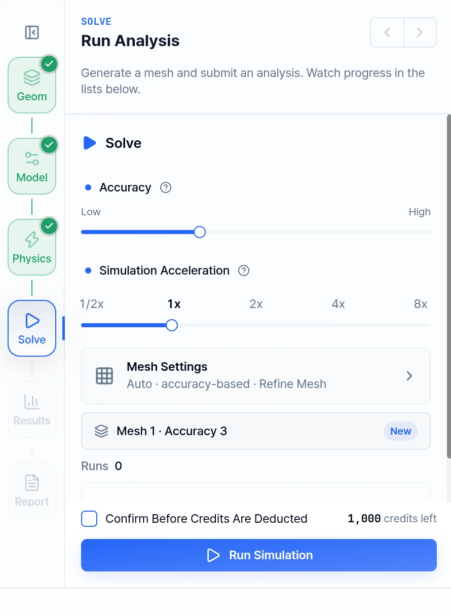
The Solve step sets the mesh and runs the analysis.
- Accuracy: A 7-step slider from Low to High. Higher accuracy gives more precise results, but takes longer and uses more credits.
- Mesh Settings: With Auto Size on, sizes follow Accuracy. With it off, the slider has no effect and you set Mesh Detail, Size Transition Smoothness, Shape Accuracy, Edge Refinement and Shape Accuracy Method (Standard, Adaptive, Precise, Maximum Precision). The toggles are Refine Mesh, Feature Smoothing and Detail Capture (Beta).
- Simulation Acceleration: 1/2x to 8x. Higher acceleration shortens the run and consumes credits faster; stops above your plan limit are locked.
Click Run Simulation to generate the mesh and solve, or Generate Mesh Only to preview the mesh first. To inspect a mesh, show it on the canvas from its mesh card and use Section View.
When solving starts, the Residuals chart opens at the bottom of the workbench. Use Residuals in the status bar to reopen it.
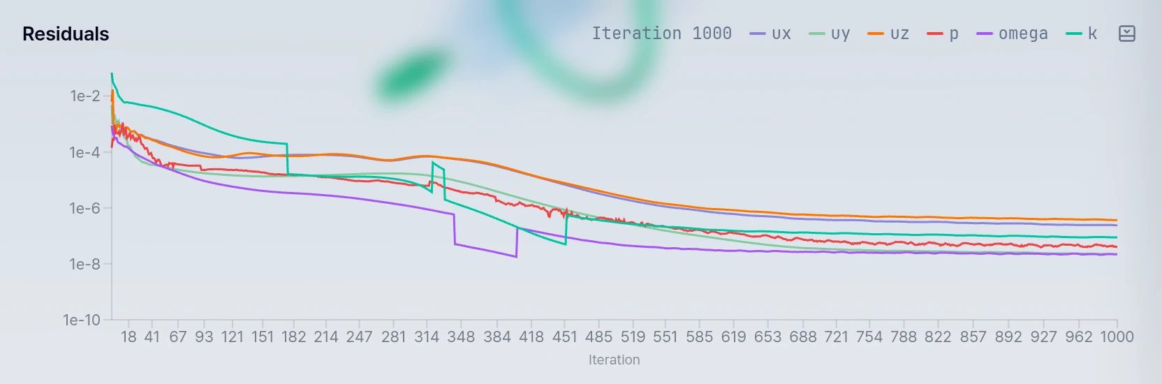
Residuals
A fundamental indicator used to evaluate the convergence of a flow simulation.
To determine whether the simulation has converged properly, the residual values of each solution variable must be sufficiently low.
7. Results (3D Contour)
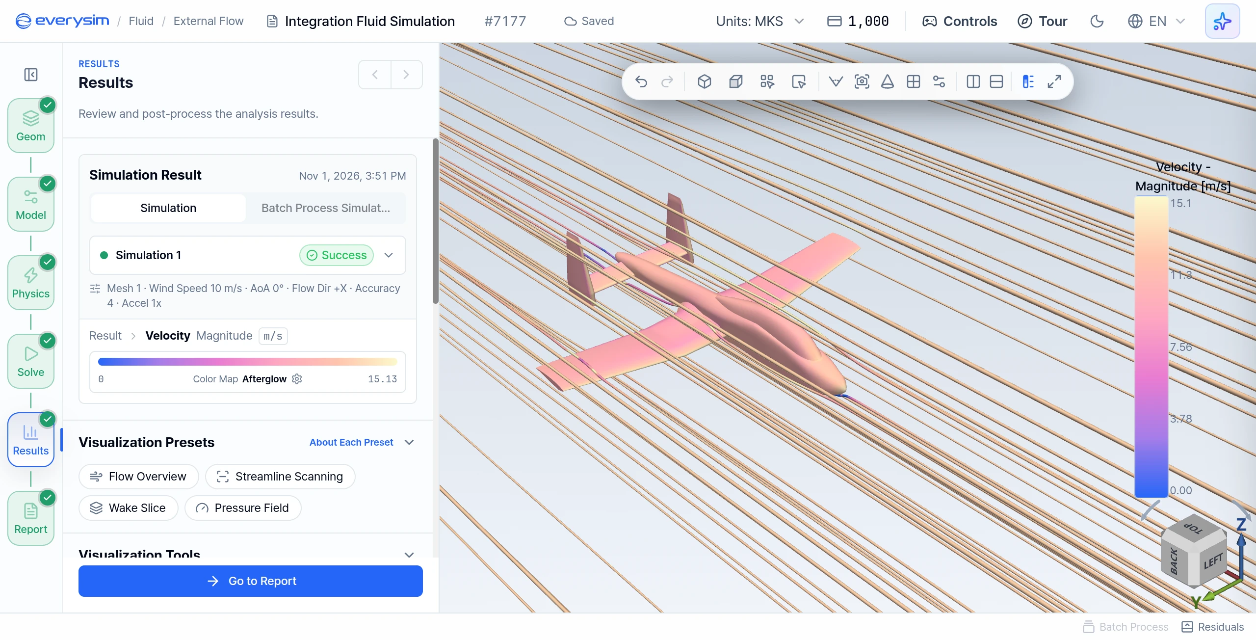
Figures 7 to 9 are from the sample model at 10 m/s and 0° angle of attack in a Wind Tunnel domain, at Accuracy 4. In Figure 7 the fluid domain is hidden by setting the Opacity of Result to 0 under Result Fields, with Streamline on and seeded by Sphere.
Results and Report unlock after a successful run.
- Results Tree: Displays Velocity, Pressure, Turbulence, Vorticity, Advanced Vorticity, Wall Shear Stress and y+.
- Visualization Presets: Flow Overview, Streamline Scanning, Wake Slice and Pressure Field each set up a common view in one click.
- Visualization Tools: Turn on Streamline to visualize the flow, seeded by Sphere or Line. The same list includes Color Map, Threshold, Isosurface, Probe, Cut and Clip.
8. Report
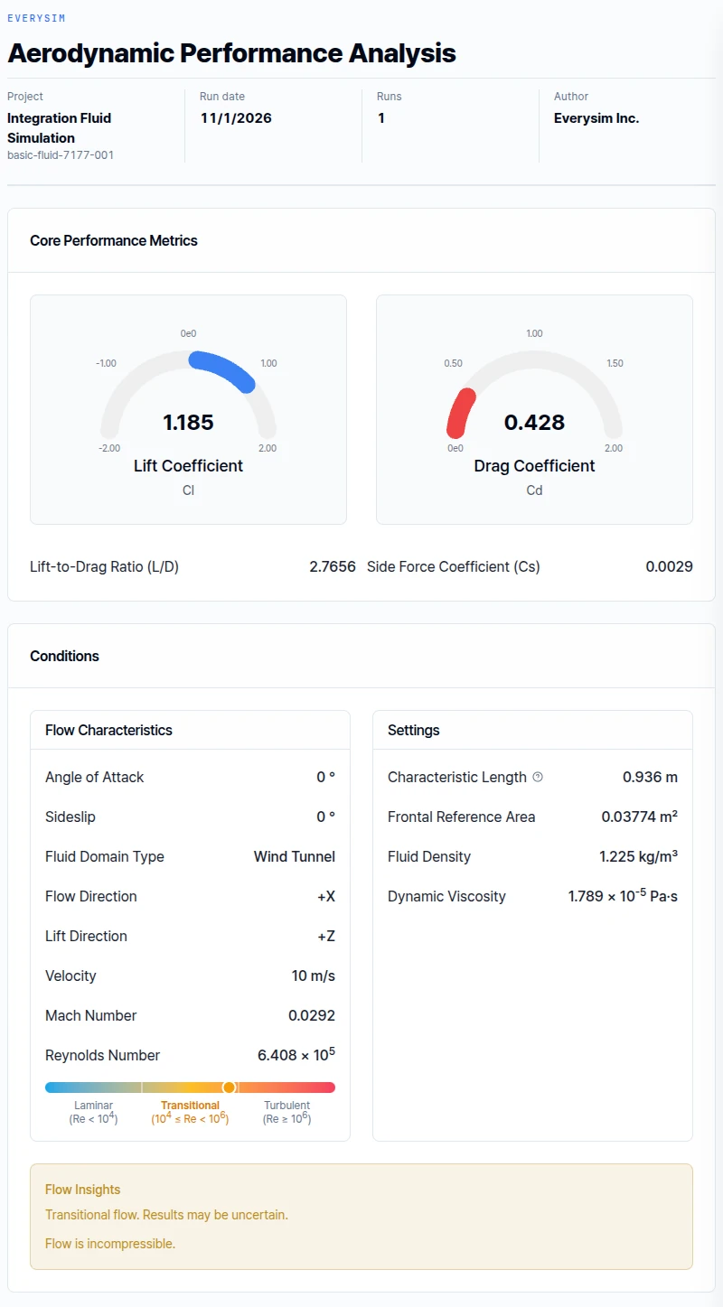
The report in Figure 8 uses the frontal area, 0.03774 m², as its reference area, with a Characteristic Length of 0.936 m. On that basis the Lift Coefficient is 1.185 and the Drag Coefficient is 0.428, for an L/D of 2.77. A coefficient based on frontal area does not compare directly with one based on wing area.
8.1. Aerodynamic Performance Analysis
Lift Coefficient (CL)
The Lift Coefficient is a dimensionless number that represents the lift force generated by the body. It is defined by the following equation:
Where:
- : Lift force
- : Fluid density (1.225 kg/m³ for default air)
- : Wind speed
- : Reference area
Drag Coefficient (CD)
The Drag Coefficient is a dimensionless number that represents the drag force acting on the body. It is defined by the following equation:
Where:
- : Drag force
- : Fluid density
- : Wind speed
- : Reference area
The report also shows the Lift-to-Drag Ratio (L/D) and the Side Force Coefficient (Cs).
Flow Characteristics
- Velocity: Equivalent to wind speed.
- Mach Number: A dimensionless quantity representing the ratio of the object's speed to the speed of sound in the surrounding medium.
- Reynolds Number: A dimensionless number representing the ratio of inertial forces to viscous forces in the fluid.
The conditions also list the Angle of Attack, Sideslip and Fluid Domain Type used in the run.
Settings
- Characteristic Length: The value set in Reference Dimensions.
- Reference Area: The area that follows from the Object Type set on the Geometry step.
- Fluid Density: 1.225 kg/m³ for default air.
- Dynamic Viscosity: A measure of a fluid's resistance to flow.
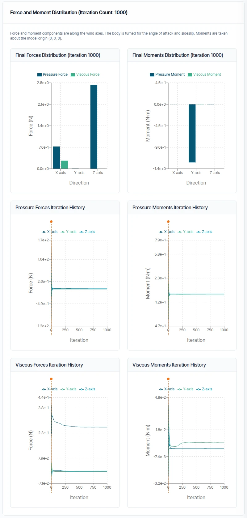
8.2. Force and Moment Distribution
- Final Forces Distribution and Final Moments Distribution: Display the forces and moments at the end of the simulation, classified into pressure and viscous components.
- Iteration History: Shows forces and moments per iteration. This provides insight into the convergence of the aerodynamic forces and moments.
Need Assistance or Have Questions?
Frequently Asked Questions: FAQ Link
Support Inquiries: support@everysim.io