4.1 Structural Analysis: Component-Propeller
1. Geometry
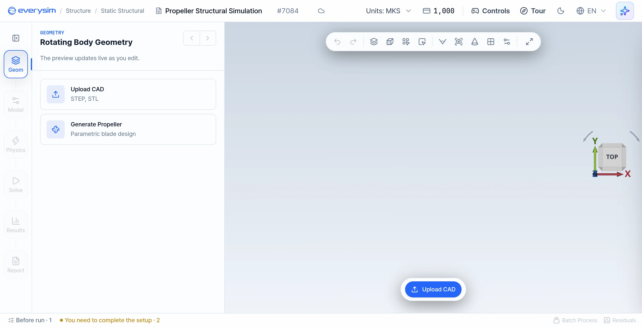
This screen shows the first step of the structural component workflow. The step rail on the left shows Geom, Model, Physics, Solve, Results and Report. The setup panel sits beside the rail, and the 3D viewport is on the right.
In Geom, choose Generate Propeller to build the blade parametrically, or Upload CAD to import your own file or the Propeller sample model. The Your Own CAD page covers the upload path.
1.1. Generate Propeller
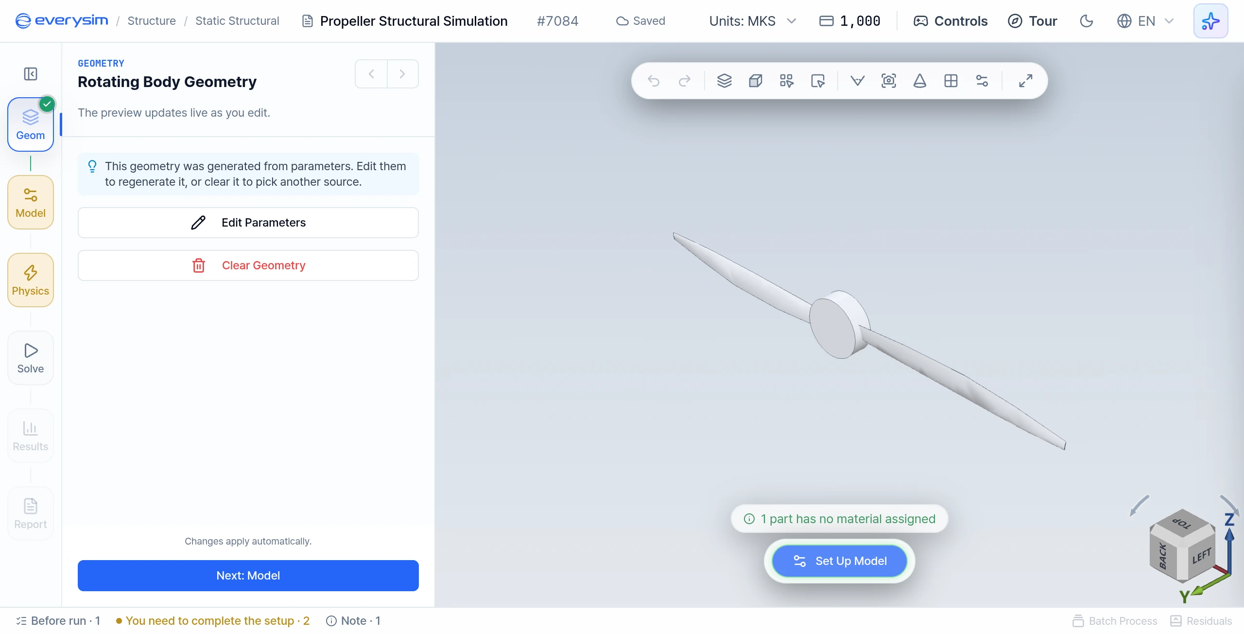
Generate Propeller opens the propeller editor with a propeller already built. Valid edits are generated and saved automatically, and the preview in the viewport updates as you type. The editor has two modes: Airfoil (default) and Parametric. This figure shows the panel after you leave the editor: Edit Parameters reopens the editor, and Clear Geometry lets you pick another source.
When the shape is right, click Next: Model at the bottom of the panel.
1.1.1. Airfoil Mode
Choose an Airfoil Profile, set Blade Count and Hub Size (×), then edit the radial Distribution. Sections lists each station with its radius (r), Chord, Twist and Pitch Axis.
1.1.2. Parametric Mode
The editor shows Blade Count, Hub Cap, the Blade Layout diagram, the section cards Root, Middle and Side, and a Hub card.
The three section cards share the same fields and define the blade shape at three positions. The angles must satisfy α+β ≤ 90.
- Length
- Angle of attack (α)
- Pitch angle (β)
- Left radius, Right radius and Center radius
- Distance
- Depth
The remaining settings define the blade count and the hub:
- Blade Count: Total number of blades
- Hub Cap: Whether to include a cap at the hub center
- Outer: Hub outer radius
- Inner: Hub inner radius
- Height: Hub height
2. Model: Material Properties
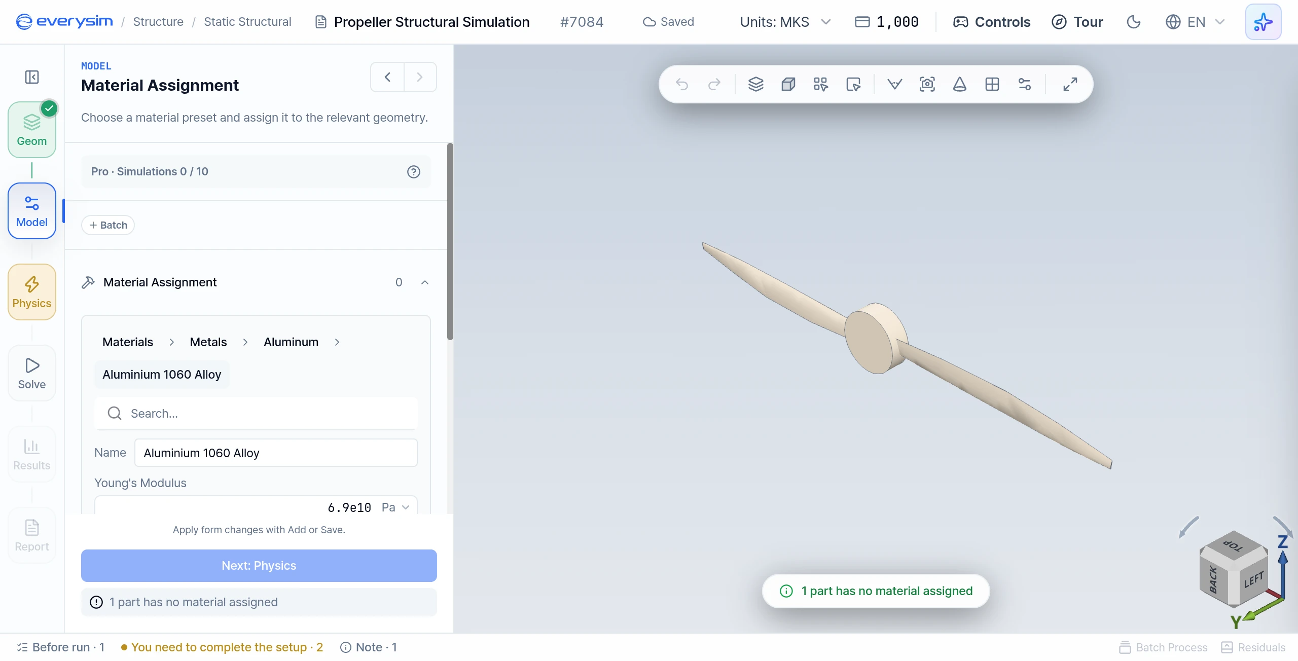
This screen shows Material Assignment in the Model step. The form is in the panel on the left, and the propeller is in the viewport on the right.
Click Add Material, then choose Materials > category > family > material, or use the search box. The categories are Metals, Plastics & Polymers, Ceramics & Glass, Natural & Biological, and Other. Metals are further split into Steel, Aluminum and Other Metals.
There is no separate manual entry mode. The fields below appear once a material is selected, so for a custom material, choose the closest preset and then edit its values:
- Name: Name of the material
- Young's Modulus: Elastic stiffness of the material (above 0)
- Poisson Ratio: Ratio between lateral and axial strain (0 to below 0.5)
- Density: Mass per unit volume of the material (above 0)
- Thermal Exp.: Thermal expansion coefficient of the material. The app has no thermal load.
- Tensile Str.: Maximum tensile stress before failure
- Yield Str.: Stress level where permanent deformation begins
A generated propeller is one body, so it is selected automatically. Check the highlighted body in the viewport, then click Add.
3. Physics: Constraints
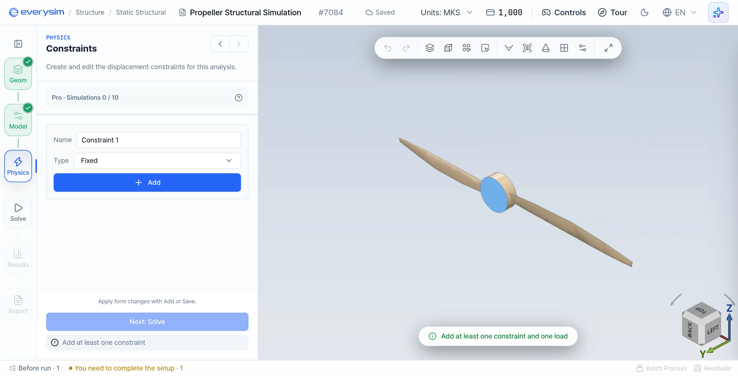
This figure shows the constraint form in the Physics step, with the selected hub faces highlighted in the viewport.
Under Constraints, click Add Constraint, then set Type to Fixed or Displacement. Click faces in the viewport (hold Shift to add more), then click Add.
3.1. Fixed
Use Fixed to lock the selected faces. This is commonly applied to the hub or mounting area to represent the part connected to the motor shaft.
3.2. Displacement
Use Displacement when a specific displacement should be applied to the selected faces.
- Dx, Dy, Dz: Displacement per axis, in the unit shown beside the field (m in the default MKS preset)
Enter * to leave an axis free. At least one axis must be constrained.
4. Physics: Loads
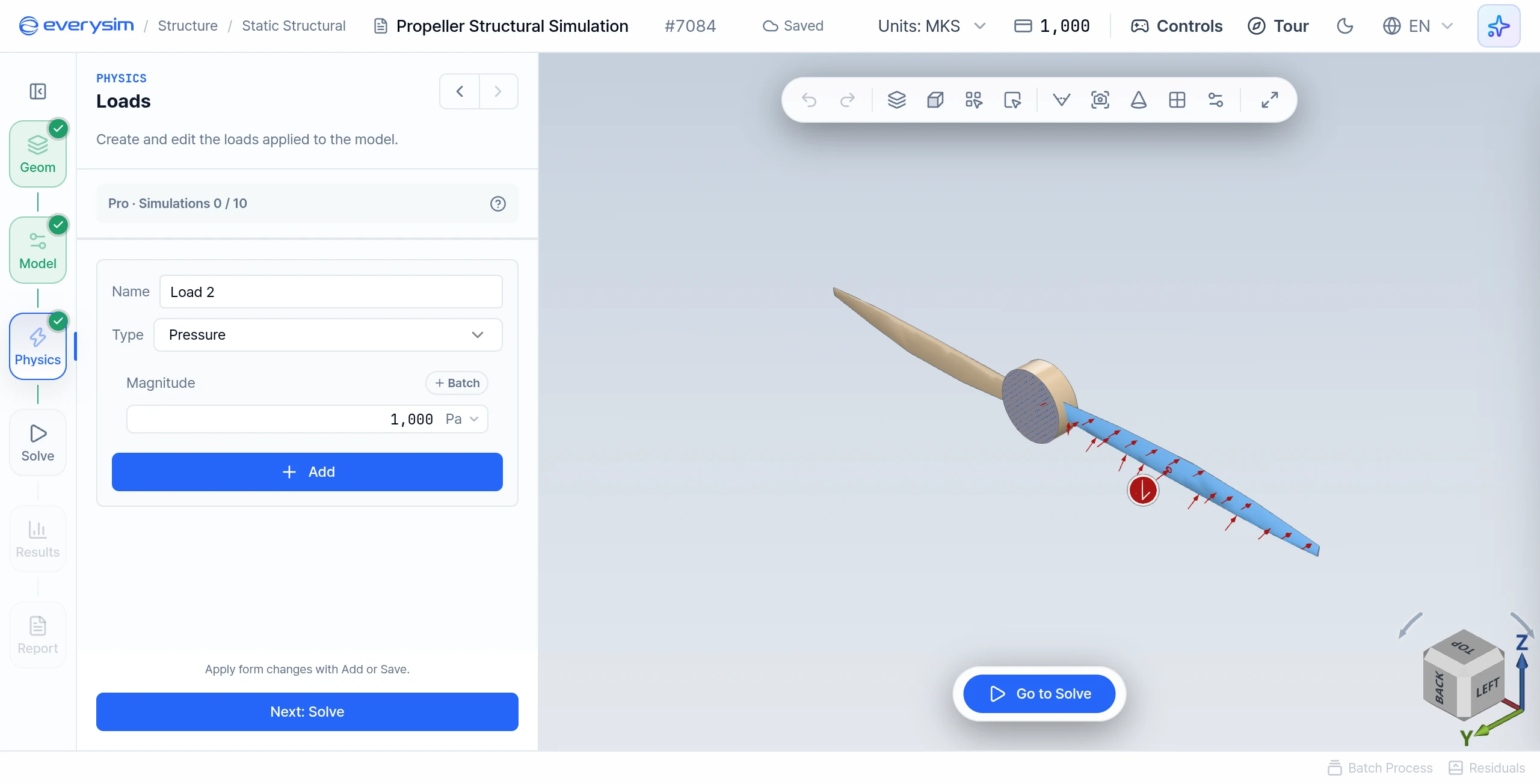
This screen shows the load form. The selected faces are highlighted in the viewport, and the load arrows show where the load acts. This step defines the external forces that the propeller will experience during the structural analysis.
Under Loads, click Add Load, then set Type to Pressure, Facial Force, Gravity or Displacement. Click faces in the viewport (hold Shift to add more), enter the values, then click Add. A run needs at least one constraint and one load.
4.1. Pressure
Use Pressure to apply a distributed load normal to the selected faces. Enter the value in Magnitude, in the unit shown beside the field (Pa in the default MKS preset).
4.2. Facial Force
Use Facial Force to apply force components directly to the selected faces.
- Fx, Fy, Fz: Force per axis, in the unit shown beside the field
4.3. Gravity and Displacement
Gravity does not need a face selection, and a model can have only one. Displacement takes the same Dx, Dy, Dz input as the displacement constraint.
5. Solve: Mesh and Accuracy
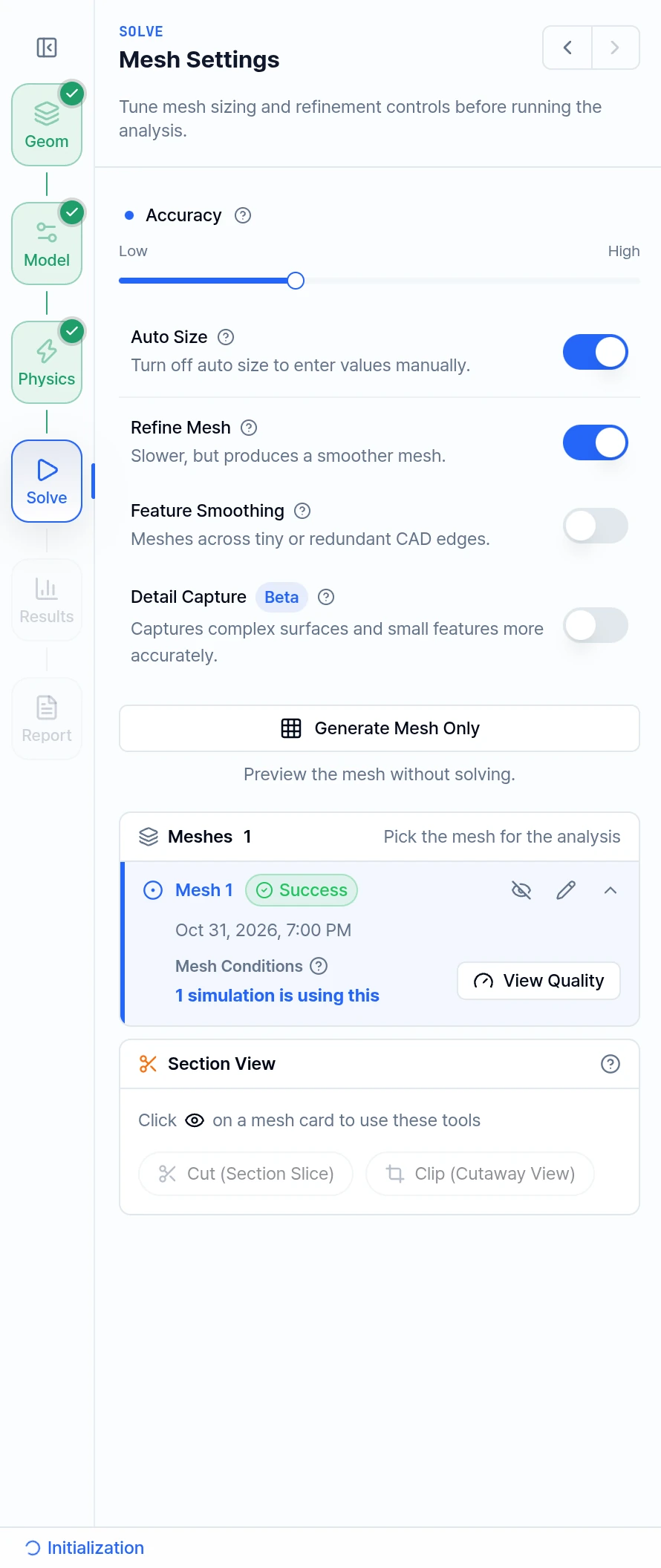
This figure shows Mesh Settings after a mesh has been generated, with the mesh listed under Meshes. These settings determine how detailed the finite element mesh will be.
Mesh setup happens in the Solve step, under the heading Run Analysis.
5.1. Accuracy
The Accuracy slider has 7 steps, from Low to High. Higher values create a finer mesh, and take longer and use more credits. Steps 1-2 may give large errors. The slider has no effect when Auto Size is off.
5.2. Mesh Settings
Click Mesh Settings to open these switches:
- Auto Size: Sizes follow the Accuracy slider. Turn it off to enter values manually.
- Refine Mesh: Slower, but produces a smoother mesh
- Feature Smoothing: Meshes across tiny or redundant CAD edges
- Detail Capture (Beta): Captures complex surfaces and small features more accurately
You don't have to generate the mesh yourself. Run Simulation generates the mesh or reuses a matching one, then solves. To inspect the mesh first, click Generate Mesh Only in Mesh Settings.
The Meshes card records mesh generation status, accuracy, and the analyses that use the mesh. A running analysis appears separately in the Runs list so mesh progress and solver progress can be reviewed independently.
The mesh is reused automatically when geometry and mesh settings are unchanged, so changing only a material or a load magnitude keeps the mesh. If they change, the next run builds a new mesh and the panel tells you so. Check that the mesh status shows Success before relying on the result.
6. Solve: Run Simulation
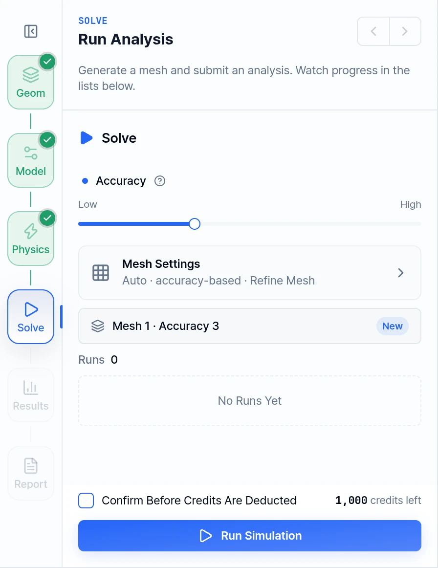
This figure shows the structural Solve panel. Structural runs have no acceleration setting, so Accuracy is the only slider here. The earlier steps are marked as complete in the step rail.
Once Geom, Model and Physics are complete, click Run Simulation to start the structural analysis job.
After the simulation finishes, review the generated results to evaluate whether the propeller can withstand the assigned constraints and loads.
7. Results
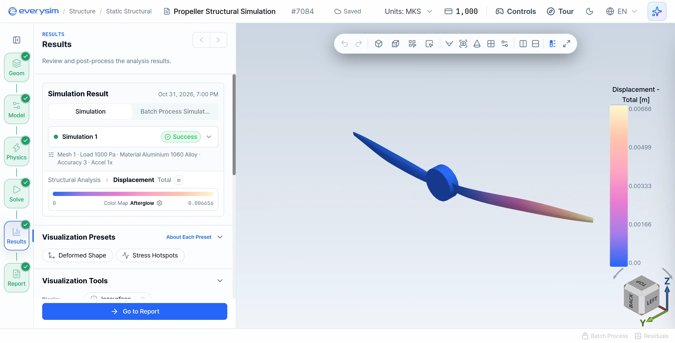
The Results stage displays the solved structural fields on the propeller and keeps the successful simulation record visible in the setup panel. The run summary lists "Accel 1x", but this is not a setting: a structural run always uses one core. Expand Structural Analysis to inspect:
- Displacement: total displacement and its X-, Y-, and Z-axis components.
- Equivalent Stress: von Mises, Tresca (Max Shear) and Signed von Mises fields.
- Principal Stress: the principal stress components at each location.
- Stress Tensor: the complete tensor representation for detailed review.
For displacement results, enable the Scale Factor when the physical deformation is too small to see at true scale. Use Play Animation to inspect the deformed shape through the displayed motion cycle. Always read the color legend and units before comparing regions.
8. Report
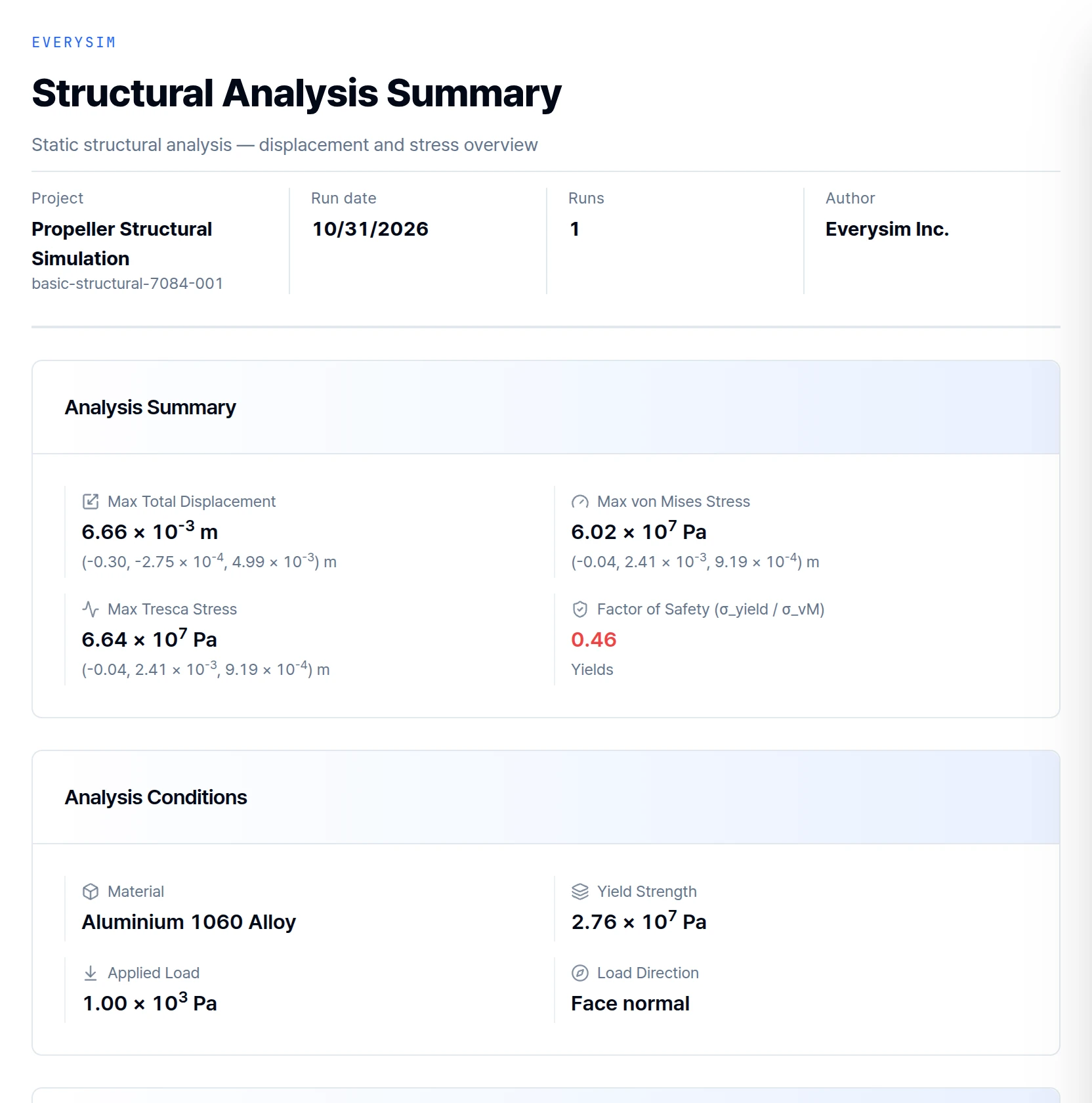
The structural report summarizes the simulation in a form that can be reviewed without manipulating the 3D result:
- Max Total Displacement: largest displacement magnitude and its location.
- Max von Mises Stress and Max Tresca Stress: peak equivalent-stress measures and their locations.
- Factor of Safety: material yield strength divided by the maximum von Mises stress. Below 1, the peak von Mises stress exceeds the yield strength and the report marks the result as Yields. Otherwise it shows Safe.
- Analysis Conditions: material, yield strength, applied load and load direction.
- Engineering Insights and Key Results: critical-node displacement components and principal stresses.
Figure 9 shows a Factor of Safety of 0.46 with the verdict Yields. This is expected for the default load used in this example: on Aluminium 1060, the peak von Mises stress of 6.02 × 10⁷ Pa exceeds the yield strength of 2.76 × 10⁷ Pa. It demonstrates how the report flags yielding, not a design you should accept.
Use the report together with the 3D result. A high factor of safety does not replace checks for realistic constraints, correct load direction, appropriate material data, and adequate mesh resolution.
Need Assistance or Have Questions?
Frequently Asked Questions: FAQ Link
Support Inquiries: support@everysim.io